Making Measurements — S11, S21, the Smith Chart, and Time-Domain Reflectometry

---

4.1 About this volume

Vol 3 closed with a calibrated, trustworthy reflection coefficient Γ sitting in the instrument’s memory at every swept frequency, and it was explicit that trustworthiness is exactly where its job ends: “what you do with that trustworthy number — reading return loss and SWR off it, walking the Smith chart, running a TDR sweep — is [Vol 4]‘s job.” This is that volume. Everything here assumes the calibration discipline Vol 3 built — a stale or mismatched-span calibration poisons every number this volume teaches you to read, and if a reading here looks wrong, the first diagnostic step is always to ask whether the calibration is still valid for the sweep in front of you, not to doubt the math below. A measurement is only as good as its calibration; this volume will not repeat that argument, only lean on it.

What this volume owns is the use of a calibrated sweep: reading an S11 trace as return loss, SWR, and — the part every operator eventually has to learn and most skip for years — as a complex impedance that tells you which of two very different problems you actually have. It owns the S21 sweep and what a “1-port-plus-transmission” instrument like a NanoVNA genuinely measures for a 2-port device. It owns phase and group delay, and the discipline of knowing when a delay number is telling you something about your feedline or matching network and when it is just amplified measurement noise. It owns the Smith-chart workflow on the device’s own screen — reading a marker, recognizing the five canonical motions a reactive element or a length of line produces, and using those motions to design a matching network by inspection rather than by algebra. And it owns time-domain reflectometry: the principle by which a frequency sweep becomes a distance-to-fault reading, and the velocity-factor arithmetic that is, without exception, the largest source of error in that reading.

The throughline connecting all of it is a single idea stated plainly here because it organizes everything that follows: a scalar SWR meter can only ever tell you that something is wrong; a calibrated vector instrument can tell you what. A return-loss dip that lands at the wrong frequency and a return-loss dip that lands at the right frequency but never gets deep enough produce nearly identical SWR-meter readings — “SWR is too high at my operating frequency” — and yet they call for opposite fixes: one is solved with a hacksaw, the other is made worse by one. Section 3 makes that distinction the centerpiece of this volume because it is, in a real sense, the entire point of owning a NanoVNA rather than an MFJ analog SWR bridge.

Three explicit boundaries with the volumes on either side of this one. Vol 1 owns the S-parameter definitions, the reflection coefficient Γ, and the bilinear Γ ↔ Z mapping that puts an impedance on a Smith chart in the first place — this volume applies that mapping constantly and rederives none of it. Vol 3 owns calibration end to end, including the sweep-span and point-count constraints on a calibration’s validity — this volume assumes a valid calibration and instead covers choosing a span and point count for a good reading, which is a related but genuinely different question, addressed in Section 2. Vol 5 owns the field workflow (when in a deployment day to sweep, at the rig end or the antenna end), the host software (NanoVNA-Saver and its companions), the ranked commercial-buy survey, and the instrument’s hard limitations (dynamic range, phase noise, microwave-band accuracy) — this volume is entirely about reading the numbers a calibrated NanoVNA hands you, on whichever model and in whichever software you’re using.

4.2 The S11 sweep in practice — span, points, return loss and SWR

Setting up an S11 sweep is two decisions before you look at a single number: how wide a frequency span to sweep, and how many points to spread across it. The span decision is the more consequential one, and the working rule is to sweep wider than the band you actually operate — typically the design band plus a comfortable margin on each side, enough that the resonance’s full V-shape is visible with flat, high-SWR shoulders on both edges of the plot rather than a curve that looks like it is still falling off one side of the screen. A sweep that shows only the bottom of the V invites the single most common beginner mistake in this whole discipline: mistaking “the SWR is falling as I approach one edge of my sweep” for “the antenna doesn’t resonate,” when the resonance is simply sitting just outside the window you chose. Widen the span until the curve turns back up on both sides before trusting a reading at all.

Point count is the resolution knob layered on top of that span, trading against sweep time the way you’d expect — more points means a slower sweep, because Vol 3’s calibration table is indexed by exactly the frequencies you swept, and a sparse grid can straddle a narrow resonance without landing a point near its true minimum. As a working rule, a modest point count (on the order of 100–200) characterizes a single HF band cleanly, since the resonance is broad relative to the span; a narrower search — a sharp filter notch, a high-Q matching network — wants several hundred points concentrated on the region of interest instead. Exact menu names and defaults vary by model and firmware, so this volume states the principle (resolution scales with points-per-unit-span, and the calibration constrains you to whatever grid you swept) and leaves the button sequence to Vol 5’s field workflow.

Once the sweep is running, the two numbers every operator reads are return loss and SWR, and they are two faces of the same measured quantity — the magnitude of the reflection coefficient |Γ| that Vol 1 defines. Return loss in decibels is RL = -20·log₁₀|Γ| — a positive number by this sign convention, growing larger as the match improves and |Γ| shrinks toward zero — and SWR is the familiar (1+|Γ|)/(1-|Γ|). The two move together but nonlinearly, and it is worth having the correspondence memorized rather than mentally converting on the fly every time:

Table 1 — Once the sweep is running, the two numbers every operator reads are return loss and SWR, and they are two faces of the same measured quantity — the magnitude of the reflection coefficient |Γ| that [Vol 1](/nanovna/vol-1/) defines. Return loss in decibels is RL = -20·log₁₀|Γ| — a positive number by this sign convention, growing larger as the match improves and |Γ| shrinks toward zero — and SWR is the familiar (1+|Γ|)/(1-|Γ|). The two move together but nonlinearly, and it is worth having the correspondence memorized rather than mentally converting on the fly every time

| Return loss | |Γ| | SWR | |---:|---:|---:| | 6 dB | 0.501 | 3.01:1 | | 10 dB | 0.316 | 1.93:1 | | 14 dB | 0.200 | 1.50:1 | | 20 dB | 0.100 | 1.22:1 | | 26 dB | 0.050 | 1.11:1 | | 30 dB | 0.032 | 1.06:1 |

The nonlinearity is the point worth internalizing: the first 10 dB of return-loss improvement buys you most of the SWR improvement a casual operator cares about (10 dB already gets you under 2:1), while the next 20 dB above that — the difference between an amateur-adequate match and a genuinely excellent one — buys comparatively little further SWR improvement and is correspondingly harder to chase. A NanoVNA reading return loss in the high 20s or low 30s of dB at resonance is reporting an antenna most operators would call essentially perfect; demanding 40 dB from a wire antenna over real ground is usually chasing measurement noise and cable-flex artifacts rather than real antenna performance. Section 3 is where the return-loss number stops being the whole story.

4.3 Reading the impedance — the length problem versus the matching problem

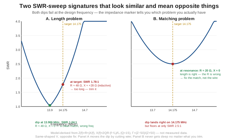
Every SWR sweep produces a single scalar summary at the frequency you care about, and that scalar is, by itself, diagnostically useless for deciding what to do next — it can only tell you that the match is bad, never why. The complex impedance sitting behind that scalar is where the diagnosis actually lives, and reading it is the one habit that separates an operator who trims an antenna in two sweeps from one who trims it for an afternoon. The lead figure sets up the two failure modes side by side because they produce a nearly identical complaint — “SWR is too high at my operating frequency” — while calling for opposite, even contradictory, fixes.

Panel A is a length problem. The resonance — the frequency at which the reactance X crosses zero — sits at the wrong place, off to one side of the design frequency, but when the sweep is read at that actual resonance the resistance R is close to the design value and the match there is excellent. In the figure’s model, the true dip sits at 13.900 MHz with R ≈ 48 Ω, X ≈ 0, and a return loss over 30 dB — a genuinely clean match — while the design target was 14.175 MHz. Read at the target frequency instead of at the true dip, the same antenna shows R ≈ 48 Ω but X ≈ +28 Ω, an inductive reactance that has walked the SWR up to 1.78:1. The diagnosis falls directly out of that reactance sign, using the same convention Vol 1 establishes for the Γ ↔ Z mapping: a positive, inductive reactance at the target frequency means the resonance you actually built sits below where you want it, which for a simple resonant element means the conductor is electrically too long — extra length adds inductive reactance below its own resonance. The fix is mechanical: trim the element, using whichever per-band trim-sensitivity figure the relevant antenna volume in this hub provides, and re-sweep. No matching-network adjustment, however cleverly chosen, moves the frequency at which X crosses zero; only changing the antenna’s own electrical length does that.

Panel B is a matching problem, and it is the case operators miss more often precisely because the SWR-meter symptom looks the same. The resonance lands exactly on the design frequency — X ≈ 0 right at 14.175 MHz, so the length is correct and no amount of trimming will move the dip anywhere, because it is already where it belongs — but the resistance at that dip is R ≈ 20 Ω rather than the intended 50 Ω, and the SWR floor never drops below about 2.5:1 no matter how precisely the sweep is centered. This is the fingerprint of a resistance mismatch: the antenna’s feedpoint impedance itself, set by height above ground, matching-network component values, ground-system quality, or antenna-family geometry (a shortened or loaded vertical’s characteristically low feed resistance is a common real-world source), sits away from 50 Ω even though the electrical length is exactly right. Trimming an antenna with this signature is worse than doing nothing — cutting or extending the element moves the resonant frequency off the one place it was already correct, trading a matching problem for a matching problem plus a new length problem, without touching the actual cause. The fix here is a matching-network adjustment, a height change, or a ground-system improvement — whatever actually sets R — never the element length.

The two-knob discipline generalizes beyond any one antenna family: whenever a build has two independent things that can be wrong (length and a separate impedance-setting parameter — a radial droop angle, a matching-network tap, a loading-coil position), the sweep-and-trim loop converges fastest by fixing frequency first with the other parameter held constant, then fixing impedance with the length now frozen — not adjusting both at once and fighting the coupling between them. Individual antenna-family volumes work a concrete version of this loop for their own geometry; this volume contributes the instrument-reading principle underneath all of them — read R and X together, every time, and let the sign and magnitude of each tell you which knob to turn.

4.4 The S21 sweep — insertion loss and what a 1-port-plus-transmission instrument gives you

A 2-port device under test — a filter, a BALUN or UNUN, a length of feedline, a matching network — needs a second measurement beyond S11, because a device can present a perfectly matched input while still throwing away most of the power that goes in, and S11 alone cannot see that. S21 is the transmission measurement: with the DUT’s input on port 1 and its output on port 2, insertion loss in decibels is IL = -20·log₁₀|S21|, and reading it is mechanically identical to reading return loss — a bigger number is a better (lower-loss) result, and the sign convention is chosen so insertion loss is reported as a positive number of decibels lost, exactly the way return loss is reported as a positive number of decibels rejected.

It is worth being precise about the architecture doing this measurement, because “2-port VNA” undersells how modest the hardware behind a NanoVNA actually is. A full-featured laboratory VNA has a directional bridge and a calibrated receiver at each port, so it can measure all four S-parameters — S11, S21, S12, S22 — from a single connection, in either direction, without touching the DUT. Much of the NanoVNA family is, at its architectural heart, closer to a 1-port instrument with a switched transmission path bolted on: one directional bridge lives at port 1, and port 2 is a second receiver that samples whatever comes through the DUT, giving you S11 and S21 from a single sweep with the DUT connected in one orientation. What that architecture does not generally give you automatically is S22 or the reverse transmission S12 — measuring those means physically reversing the DUT (swapping which end is on port 1) and sweeping again, because there is no second directional bridge sampling reflections at port 2 the way there is at port 1. This is not a defect, just an honest description of a one-bridge instrument, and it is why “1-port-plus-transmission” is a more accurate mental model than “2-port VNA” for much of this family — Vol 5’s per-model survey covers which current units add the second bridge.

For amateur measurement work this limitation rarely bites, because the DUTs of interest — filters, BALUNs, feedline sections, matching networks — are frequently close to reciprocal and the forward measurement (S11 and S21 with the DUT in its normal operating orientation) is the one that actually matters operationally. Reading an S21 trace, a clean passband shows a magnitude close to 0 dB (allowing for the DUT’s real insertion loss — a well-built 1:1 current BALUN or a short run of low-loss coax should sit within a fraction of a decibel of flat) with a smoothly rolling phase; a filter’s stopband shows the magnitude falling away by tens of decibels beyond the cutoff, and the frequency at which the magnitude has fallen 3 dB from its passband value is the conventional cutoff-frequency marker, the same −3 dB convention every other bandwidth discussion in this hub uses. A device that shows unexpectedly high insertion loss in what should be a clean passband is showing you real loss — resistive loss in a lossy core, a poor connector, water in a connector body — and not a calibration artifact, provided the through-line calibration Vol 3 describes was actually performed; skip that step and the cable’s own loss gets folded into every S21 reading indistinguishably from the DUT’s.

4.5 Phase and group delay — signal and noise

S21 carries a phase alongside its magnitude, and that phase is a second, independent channel of information about the DUT that a magnitude-only measurement throws away entirely. The most direct thing phase measures is electrical length: a matched, lossless length of transmission line produces a phase that is exactly linear in frequency, φ(f) = -2π f · ℓ / v_p, where ℓ is the physical length and v_p is the propagation velocity — Section 9 develops v_p in terms of velocity factor. A linear phase slope is, in other words, the signature of “this is just a length of line,” and it is genuinely useful: measuring the slope of an S21 phase sweep through a run of feedline, and knowing the velocity factor, gives you an independent check on the feedline’s physical or electrical length without cutting it open or trusting a spec-sheet number for a batch of unknown-provenance coax.

Group delay is the derivative form of that same information, τ_g = -dφ/dω, in units of time. A pure length of matched line has constant group delay — flat with frequency, equal to ℓ/v_p — the signature of “nothing frequency-selective here, just a length of line.” A frequency-dependent delay instead signals something reactive and resonant doing work — a matching network, a filter, an antenna near its own resonance — because a resonant structure’s phase bends most sharply right where it is doing the most reactive work, which for a network tuned to a specific frequency is right around that frequency. A narrowband resonator’s delay peaks at its own center frequency and falls away on either side, with the peak height and sharpness set by Q — exactly the same relationship the Single-Band Dipoles dive develops between Q and 2:1-SWR bandwidth, read through a different instrument mode.

The figure below computes group delay through a representative narrowband two-pole resonator at f₀ = 14.175 MHz with Q ≈ 8 — illustrative, and deliberately not Section 7’s specific L-match, whose loaded Q = √(50/20 − 1) ≈ 1.22 would give a peak of only about 27 ns and would barely rise above the flat reference at all by differentiating its phase numerically, checked against the closed form τ_g(f₀) = Q/(π f₀) at resonance. The peak of roughly 180 ns at f₀, falling to under 50 ns a megahertz away, sits against a flat 50 ns reference representing about 12.7 m of ordinary feedline (LMR-400, the velocity factor Section 9 uses) — flat means length, peaked means resonance.

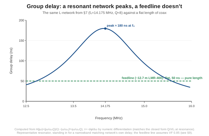
This distinction has two practical uses and one trap. It matters for establishing a feedline’s electrical length independently (flat delay, read the value, multiply by v_p) and for judging whether a matching network’s bandwidth is narrow enough to distort a wideband digital-mode signal (a peaked, high-Q curve says yes; broad and low-Q says no). It is noise, not signal, whenever the delay trace itself looks jagged rather than the underlying phase — group delay is a numerical derivative of an inherently noisy phase measurement, and differentiation amplifies noise: phase jitter invisible on a magnitude plot becomes a visibly ragged delay curve once you take its slope. Averaging more sweeps or using more points is a more productive response than concluding the DUT has real jagged delay at that resolution.

4.6 The Smith-chart workflow — the canonical trajectories

Vol 1 established the bilinear mapping Γ = (z-1)/(z+1) (with z = Z/Z₀ the impedance normalized to the system reference, ordinarily 50 Ω) that puts every possible impedance somewhere inside the unit circle of the Γ-plane, and the constant-resistance circles and constant-reactance arcs that make that plane readable as a chart rather than an abstract complex-number plot. This volume assumes that mapping and puts it to work: switching the device’s display to Smith-chart mode turns the same calibrated S11 sweep from Section 2 into a trace across that chart, and a marker on the trace reads off R and X directly — the real and imaginary parts of the impedance at that marker’s frequency — from whichever constant-resistance circle and constant-reactance arc the point sits on.

What makes the chart worth using for more than a pretty display is that adding a simple reactive element always moves the point along one of exactly two families of curve, and knowing which family you’re on tells you immediately what kind of element gets you where you want to go. A series element changes only the reactance, never the resistance, so it slides the point along the constant-resistance circle it started on — a series inductor toward more positive reactance (up, inductive), a series capacitor toward more negative reactance (down, capacitive), never crossing to a different constant-R circle. A shunt element does the mirror-image thing in the admittance domain: it changes only susceptance, never conductance, sliding the point along a constant-conductance arc that looks like none of the circles printed on the chart, since it belongs to the admittance grid — computed by converting to Y = 1/Z, adding the susceptance, and converting back. A shunt inductor adds negative susceptance, a shunt capacitor positive, by the standard convention. The fifth motion belongs to neither family: a length of matched line rotates Γ at constant magnitude — constant SWR — around the chart’s exact center, by an angle 2βℓ proportional to electrical length, the same rotation Vol 3’s reference-plane discussion uses to move a calibrated answer between physical locations. A quarter-wavelength is a 180° rotation — a straight-through reflection across the center — the fact behind every quarter-wave-transformer result elsewhere in this hub.

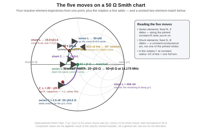
The figure below draws all five motions from one shared starting point, Z = 30 + j20 Ω, with every endpoint computed from the formulas above rather than sketched by eye: a series inductor moves the point up the constant-R = 0.6-normalized circle to 30 + j40 Ω; a series capacitor moves it down the same circle to 30 + j0 Ω; a shunt inductor and a shunt capacitor each move it along a constant-conductance arc computed through the admittance domain, landing at 19.6 + j21.6 Ω and 41.1 + j9.6 Ω respectively for the specific susceptance step used here; and λ/12 of line rotates the point 60° around the chart’s center at constant |Γ|. None of these five endpoints are arbitrary illustrations — each is the literal result of applying the stated formula to the stated starting point, which is the only way a Smith-chart figure earns the right to be trusted rather than merely admired.

4.7 Designing a match on the chart, by inspection

The payoff for recognizing those five motions is that designing a two-element L-network match — the most common matching topology this hub uses throughout the antenna and matching-network volumes — becomes a graphical procedure rather than an algebraic one, and the same figure above carries a complete worked example through it. Take a DUT presenting Z_L = 20 - j20 Ω at 14.175 MHz — a plausible low-R, capacitive feedpoint, the sort a shortened vertical often shows — and the goal is a two-element network that transforms it to 50 + j0 Ω.

The rule that decides which element goes first falls directly out of the geometry Section 6 just established. The constant-resistance circles are all mutually tangent at the chart’s open-circuit point, which means a series element alone can never move you from one resistance value to another — it can only slide you along the one constant-R circle you’re already on. The circle you land on after a series-only move can, however, cross the admittance chart’s unity-conductance circle (the arc that a shunt element can then ride the rest of the way to the match), and whether it does depends on whether the load’s normalized resistance is below or above 1. For r_L = 20/50 = 0.4 < 1, the constant-r = 0.4 circle does cross the unity-conductance circle at a finite reactance, so a series element first, then a shunt element, is the topology that works; had the load’s resistance been above Z₀ instead, the shunt-first, series-second order would be the one that closes.

Solving for where the series step should land is one line of algebra: the series element only changes X, so the question is what value of X' makes the resulting impedance 20 + jX' sit exactly on the unity-conductance circle, i.e. gives that impedance a real admittance part of 1/50 S. Writing R/(R² + X'²) = 1/Z₀ with R = 20 Ω and solving gives X'² = 50·R - R² = 1000 - 400 = 600, so X' = ±24.495 Ω. The load already sits at X = -20 Ω, so the smaller correction is the capacitive solution: a series capacitor contributing an additional -4.495 Ω of reactance, landing the point at 20 - j24.495 Ω — exactly on the unity-conductance circle, as the algebra promised. At 14.175 MHz that reactance corresponds to a capacitor of about 2.5 nF (C = 1/(ω·|X|), with ω = 2π·14.175 MHz) — a physically large value for an HF matching capacitor precisely because the correction needed here was a small one, a reminder that this component-value arithmetic is the literal algebraic result of this specific example and not a template to copy for a different load.

Converting that intermediate impedance to admittance, Y = 1/(20 - j24.495) = 0.02 + j0.0245 S, shows a residual normalized susceptance of about +1.22 that a shunt element now has to cancel by sliding along the unity-conductance arc the rest of the way to the chart’s center. Since the residual susceptance is positive (the standard convention for a capacitive admittance), the shunt element needed to cancel it is inductive — a shunt inductor contributing -0.0245 S of susceptance, which at 14.175 MHz works out to roughly 458 nH. The finished network — a small series capacitor followed by a shunt inductor — takes 20 - j20 Ω to 50 + j0 Ω exactly, and the figure’s path from the red load point through the purple series-C arc, along the shunt-L arc, to the green matched point at the chart’s center is the same two-step geometric procedure every L-network design in this hub ultimately performs, whether or not the volume in question shows its Smith-chart work. The value of doing it this way rather than by pure algebra is diagnostic as much as computational: a marker trace that visibly isn’t converging toward the center after your first element tells you, immediately and without further calculation, that you picked the wrong topology (series-first when shunt-first was needed, or the wrong reactance sign) rather than merely that your component value was off.

4.8 Time-domain reflectometry — the principle

Every measurement so far in this volume has been in the frequency domain — a magnitude and phase at each swept frequency. TDR mode takes that same calibrated frequency sweep and synthesizes an approximation of the cable’s time-domain step or impulse response from it, displaying the result as reflection amplitude against elapsed round-trip time, which the instrument then converts to distance using an assumed propagation velocity. No new physical measurement takes place to produce a TDR trace — the same S11 sweep this volume has already covered is simply transformed, mathematically, from the frequency axis it was actually swept on to a time (and then distance) axis, using the same Fourier-transform relationship that links any frequency-domain and time-domain representation of the same signal.

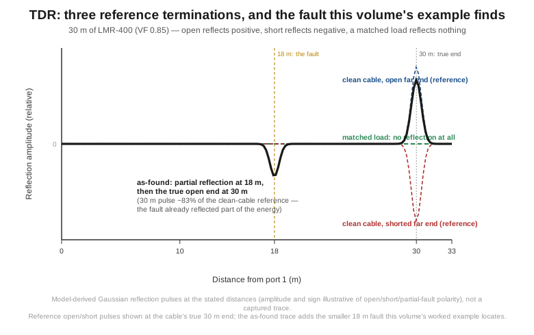
What that transform actually shows you is a signed pulse at every distance where the cable’s characteristic impedance changes — a discontinuity is, by definition, exactly what produces a reflection, and the sign and size of the pulse tell you the nature of the discontinuity. An open circuit reflects the incident wave in phase (Γ = +1), and shows up as a strong positive-going pulse at the corresponding distance; a short circuit reflects it inverted (Γ = -1), showing a strong negative-going pulse; a load that is genuinely, purely 50 Ω reflects essentially nothing, and a well-matched termination shows a flat trace with no pulse at all. A partial discontinuity — a corroded connector, a kinked or crushed section, water intrusion changing the local dielectric, a bad splice — reflects only part of the incident wave and shows a smaller pulse of whichever sign matches whether the local impedance discontinuity looks locally more like a short (impedance dropped) or more like an open (impedance rose). This is the practical value of the mode: a healthy cable terminated in an open (as it appears once you disconnect the antenna, the standard TDR-fault-finding setup) shows one clean, strong pulse at its true physical end and nothing before it; a damaged cable shows a smaller intermediate pulse at the fault’s location, followed by the same end-of-cable pulse — smaller than it would otherwise be, since the fault has already reflected away some of the energy that would otherwise have reached the true end.

The distance resolution of a TDR sweep is set by the frequency span the underlying S11 sweep covered, through the same time-frequency uncertainty relationship that governs any Fourier-based instrument: the synthesized time-domain pulse has a width on the order of 1/Δf, where Δf is the swept frequency span, so a wider frequency sweep produces a narrower, better-resolved pulse and correspondingly finer distance resolution — converting that time resolution to a distance resolution costs a further factor of the propagation velocity and the round-trip factor of two, giving approximately Δd ≈ (v_p)/(2Δf). A narrow, HF-only frequency sweep resolves distance coarsely; a sweep spanning well up into the VHF/UHF range, even on a cable that will only ever carry HF signal, resolves a fault to a substantially tighter distance window, because the resolution is set by the span of the TDR characterization sweep, not by the frequency the cable is meant to operate at. This is a real and useful practical tactic — sweep wider than your operating band specifically to sharpen a TDR search — that costs nothing but sweep time.

4.9 The velocity-factor problem — where the TDR error hides

Every distance a TDR mode reports comes from one arithmetic step: a measured round-trip travel time, multiplied by the assumed propagation velocity, divided by two for the round trip. The propagation velocity is v_p = VF · c, where c is the speed of light in vacuum and VF, the velocity factor, is the fraction by which the cable’s dielectric slows the wave relative to free space — and the velocity factor is a number you supply, not one the instrument measures. Every other input to a TDR calculation is something the instrument determines from its own sweep; VF is a property of the specific cable that has to be entered correctly by the operator, and getting it wrong scales the reported distance by the exact ratio of the wrong-to-right factor — a systematic, not random, error that silently and consistently biases every distance the sweep reports.

Velocity factor is not a universal property of a cable’s marketing name — “RG-58” or “RG-8X” — but a specific property of the actual dielectric and construction a given manufacturer ships under that name, and the honest way to use a VF number is to quote the specific cable and the specific source it came from, rather than treating “RG-58 is 0.66” as a physical constant. Three concrete, checked figures, quoted exactly as published:

• Belden 8259 (a PVC-jacketed RG-58-type cable, PE dielectric) lists a Nom. Velocity of Prop. of 66% on its own current technical datasheet.
• Belden 9258 (a PVC-jacketed RG-8X-type cable, foam-PE dielectric) lists a Nom. Velocity of Prop. of 82% on the same manufacturer’s datasheet series.
• The LMR-400 specification sheet (Times Microwave Systems’ cable data, as republished by Pasternack) lists a Velocity of Propagation of 85%, alongside a stated nominal time delay of 1.2 ns/ft that is the same number expressed the other way around.

These three numbers differ meaningfully — 66%, 82%, 85% — and every one of them is a real, published, cable-specific figure rather than a rule of thumb; a foam or air-spaced dielectric slows the wave less than solid PE, which is the physical reason LMR-400’s foam construction outpaces RG-58’s solid-PE construction by nearly 20 percentage points. Other cable types (foam-dielectric hardline, air-dielectric Heliax-class cable, differently-constructed RG-8X from a different manufacturer) will carry their own figures, and this volume deliberately does not extend the table beyond the three checked here — quoting a number this volume did not verify against a real datasheet would be exactly the fabrication-by-interpolation failure this hub’s authoring discipline exists to avoid. When in doubt, the manufacturer’s own current datasheet for the specific reel of cable in hand is the only trustworthy source; a VF pulled from memory, from a decades-old handbook table, or from a different manufacturer’s cable of the same nominal type is a plausible-looking number that may not describe the cable actually under test.

Section 10 turns this into arithmetic: because the reported distance scales linearly with the assumed VF, entering the wrong one of these three real numbers for a cable that is actually a different one of the three produces an error you can compute exactly, in advance, without needing a second measurement to discover it.

4.10 A worked example — finding a fault in 30 m of coax

Take a concrete, worked case: 30.0 m of LMR-400 running from a shack to an antenna, showing symptoms of a degraded match, with a suspected fault somewhere along its run. Following Section 8’s standard TDR fault-finding setup — disconnect the antenna, leaving the coax open at its far end — the only two reflections the sweep should show are the fault itself (if there is one) and the clean open at the cable’s true physical end.

Using LMR-400’s checked velocity factor of VF = 0.85 (Section 9) and the speed of light c = 2.998 × 10⁸ m/s, a reflection at a true physical distance d arrives after a round-trip time t = 2d/(v_p) = 2d/(VF·c). Suppose the fault sits 18.0 m from the connected end and the cable’s true physical end is, as specified, 30.0 m out. Working the formula forward — which is what the instrument’s firmware does internally, in reverse, to turn a measured time into a displayed distance — the fault’s reflection arrives at a round-trip time of 141.3 ns, and the true end’s reflection arrives at 235.5 ns. Entered correctly, with VF = 0.85 set in the instrument, those two times display directly as 18.0 m and 30.0 m, and the trace in the figure below shows exactly this: a smaller partial-reflection bump at 18 m — consistent with a partial discontinuity such as a pinched jacket or a section of moisture ingress, rather than a clean short — followed by the larger, cleaner pulse marking the true open end at 30 m.

Now suppose the operator sets the wrong velocity factor — a plausible and common mistake, since many NanoVNA firmware TDR modes offer a short menu of named cable types rather than a free-entry percentage, and picking “RG-58” from that menu for a run of LMR-400 is an easy slip when the two happen to sit next to each other in a list. The instrument still measures the same two round-trip times correctly — 141.3 ns and 235.5 ns — because that measurement doesn’t depend on the VF setting at all; only the distance it reports depends on VF, and it depends on it linearly: d_displayed = d_actual · (VF_assumed / VF_actual). The table below works this out for each of the three checked velocity factors from Section 9, entered as if it were the true value for this LMR-400 run:

Table 2 — Now suppose the operator sets the wrong velocity factor — a plausible and common mistake, since many NanoVNA firmware TDR modes offer a short menu of named cable types rather than a free-entry percentage, and picking "RG-58" from that menu for a run of LMR-400 is an easy slip when the two happen to sit next to each other in a list. The instrument still measures the same two round-trip times correctly — 141.3 ns and 235.5 ns — because that measurement doesn't depend on the VF setting at all; only the distance it reports depends on VF, and it depends on it linearly: ddisplayed = dactual · (VFassumed / VFactual). The table below works this out for each of the three checked velocity factors from Section 9, entered as if it were the true value for this LMR-400 run

VF entered	Displayed distance to the fault	Error
0.66 (Belden 8259, RG-58-type)	14.0 m	−4.0 m (−22.4%)
0.82 (Belden 9258, RG-8X-type)	17.4 m	−0.6 m (−3.5%)
0.85 (LMR-400, correct)	18.0 m	exact

Mistaking LMR-400 for RG-58 — a 19-percentage-point VF error — puts the reported fault distance more than 4 m short of its true location, a genuinely operationally significant miss if the goal is finding a specific splice or connector along a real cable run buried in a wall or run along a tower leg. Mistaking it for RG-8X is a smaller, but still real, 3.5% miss. This is the single largest source of error in any TDR distance reading a NanoVNA will ever produce — larger, in ordinary practice, than the frequency-domain-to-time-domain resolution limit Section 8 describes, larger than any residual calibration imperfection Vol 3 covers, and entirely avoidable by the simple discipline of confirming the actual cable type in hand against its actual manufacturer datasheet before trusting the displayed number, rather than assuming a menu default or a remembered rule of thumb describes the specific reel on the bench.

4.11 Where this volume hands off

This volume turned Vol 3’s trustworthy, calibrated Γ into the readings an antenna and matching-network builder actually uses. It covered the S11 sweep’s practical setup — span wide enough to see the full resonance shape, points enough to resolve it — and the return-loss/SWR correspondence, before making the case that the scalar SWR number is diagnostically incomplete on its own: the same elevated-SWR complaint splits into a length problem (resonance shifted, resistance fine at the true dip) and a matching problem (resonance on-target, resistance wrong even there), distinguishable only by reading the complex impedance, and calling for opposite fixes. It covered the S21 sweep, the honest “1-port-plus-transmission” architecture behind most of this instrument family, and phase and group delay — flat delay meaning a simple length of line, a peaked delay meaning a resonant structure doing real reactive work at that frequency, and a jagged delay trace usually meaning differentiation amplifying phase noise rather than the DUT doing anything unusual. It applied Vol 1’s Γ ↔ Z mapping to the five canonical Smith-chart motions — series L, series C, shunt L, shunt C, and a rotating transmission line — and used them to design a complete two-element L-network match by inspection, with every component value in the worked example the literal algebraic output of the formulas shown rather than a template number. And it covered time-domain reflectometry from first principles through to a complete worked fault-location example, with the central lesson that the velocity factor an operator enters, not any property of the instrument itself, is the dominant source of error in the distance a TDR sweep reports.

Vol 5 is where this all goes to work in the field: when in a deployment day to sweep, at the rig end or the antenna end, which host software logs and overlays these traces, the ranked commercial-buy survey, and the instrument’s hard limitations — dynamic range, phase noise, microwave-band accuracy — that bound every number read here. Every antenna-family and matching-network volume across this hub leans on this volume’s S11 and S21 reading discipline for its own build-and-verify loop, without re-deriving it. For the transmission-line theory behind velocity factor itself — why a dielectric slows a wave — see the Transmission Lines and Feedlines volume; for the BALUN and UNUN S21 and common-mode-rejection measurements this volume’s S21 discipline supports, see the BALUNs and UNUNs dive.

4.12 Resources

• Pozar, Microwave Engineering — the standard academic reference for S-parameter theory, the Smith chart’s bilinear construction, and the Fourier relationship between a swept frequency-domain measurement and a synthesized time-domain (TDR) response.
• Belden — technical datasheets for cable 8259 (RG-58-type) and cable 9258 (RG-8X-type) — the source verified for the two Belden velocity-factor figures (66% and 82% respectively) quoted in Section 9.
• Times Microwave Systems — LMR-400 cable specification (as republished in Pasternack’s product datasheet series) — the source verified for the 85% velocity-of-propagation figure quoted in Section 9, alongside the corresponding 1.2 ns/ft nominal time delay.
• Keysight (formerly Agilent/HP) application notes on network-analyzer measurement fundamentals — the standard industry-level treatment of insertion loss, group delay, and time-domain analysis via a swept-frequency instrument, applicable to the NanoVNA at the amateur level this volume needed.
• ARRL Antenna Book (25th+ ed.) — the amateur-facing treatment of Smith-chart matching-network design and TDR-based feedline fault-finding that this volume’s worked examples parallel.
• NanoVNA users group: https://groups.io/g/nanovna-users — active community forum, including TDR and Smith-chart usage discussions.
• NanoVNA-Saver GitHub: https://github.com/NanoVNA-Saver/nanovna-saver — the host-side software that can log and overlay the S11, S21, and TDR traces this volume describes; the full workflow for using it lives in Vol 5.
• Vol 1, Vol 3, and Vol 5 of this dive — the S-parameter and Γ↔Z theory, the calibration discipline, and the field workflow this volume builds on and hands off to, respectively.