What a Balun Actually Does

---

1.1 About this volume

This is the most cross-linked-into dive in the series, and it earns that position by sitting at a boundary every antenna has to cross. Every radiating structure in the wire-and-air cluster ends at a feedpoint. On one side of that feedpoint is an antenna with whatever impedance its geometry gives it — 25 Ω for a tightly-coupled Yagi driven element, 73 Ω for a canonical dipole, several thousand ohms for the end of a half-wave wire. On the other side is 50 Ω coaxial cable, which is unbalanced by construction and identical on every band. Something has to live in between.

That something is a balun or an unun, and the reason the family needs a whole dive rather than a paragraph is that the two words hide two genuinely different jobs. One is balance — stopping the outside of the coax shield from becoming part of the antenna. The other is impedance transformation — presenting the rig with 50 Ω when the antenna is not 50 Ω. Some devices do one, some do the other, and some do both; the failure mode that fills forum threads is an operator buying a device that solves the problem they do not have.

This volume does the first job’s theory and defers the second. It builds the common-mode problem from the three currents that can exist on a coaxial line, shows why the third one is not an imperfection but a direct consequence of connecting an unbalanced line to a balanced load, and establishes the mechanism — choking impedance — by which a ferrite core suppresses it. Then it does the thing the seed material for this dive did not: it takes seriously the finding that a high-impedance choke is not automatically a good choke, and that a choke whose impedance is reactive rather than resistive can, for entirely ordinary feedline lengths, increase the common-mode current it was installed to reduce.

The topology that implements all of this — Guanella, Ruthroff, transmission-line transformer, autotransformer — is Vol 2. The core material that determines whether the choking impedance is resistive where you need it is Vol 3. The five canonical ratios and the antennas that need them are Vol 4. The winding recipes, the bench verification, and the commercial survey are Vol 5.

A note on what this volume is not. It is not a survey of received wisdom. Several of the most-repeated rules about baluns — that more choking impedance is always better, that the required impedance is some multiple of the load impedance, that a common-mode choke and a balun are interchangeable — do not survive contact with the measurements, and where they do not, this volume says so and cites who measured it.

1.2 The three currents on a coaxial feedline

Start with the cable, before any antenna is attached. A coaxial line has two conductors: a centre conductor and a shield. It is natural to expect two currents. There are three, and the third is the entire subject of this volume.

The reason is skin effect. At HF the current in a conductor flows in a thin surface layer — a few micrometres of copper at 14 MHz — and the shield of a coaxial cable has two surfaces: an inner one facing the centre conductor, and an outer one facing the world. Those two surfaces are, at radio frequency, electrically distinct. Current on one does not imply current on the other. So the complete inventory is:

1. The current on the centre conductor, I₁. The wanted signal.
2. The current on the inner surface of the shield, I₂. Equal in magnitude to I₁ and opposite in direction, because the two form a transmission line: the fields are entirely contained in the dielectric between them.
3. The current on the outer surface of the shield, I₃. Unwanted, unaccounted for by transmission-line theory, and free to be anything the external circuit allows.

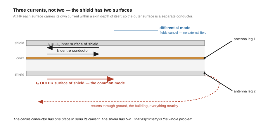
The pair I₁ and I₂ is called the differential mode (or transmission-line mode). It is well-behaved: because the two currents are equal and opposite and the geometry is coaxial, the external magnetic field of the pair is zero. A coaxial line carrying only differential-mode current does not radiate, is not affected by what it runs past, and can be bent, buried, or coiled without consequence. This is the whole reason coax exists.

I₃ is the common-mode current, and it has none of those properties. It flows on the outside of the shield, which is just a wire in space. A wire in space with current on it radiates, receives, and couples to everything near it. The feedline stops being a feedline and becomes part of the antenna.

Two consequences follow immediately and are worth stating plainly because they are frequently muddled.

First, the differential and common modes are independent. They can be analysed separately and superposed. A device can be transparent to one and opaque to the other — which is exactly what a current balun is, and exactly why it works.

Second, the common-mode current is not leakage through the shield. Braid transparency and shield effectiveness are a separate topic; a solid-copper semi-rigid line with no leakage whatsoever carries common-mode current just as happily as cheap RG-58. The third current is a property of the outside of the shield, and no amount of shielding integrity addresses it.

1.3 Where the third current comes from

The usual framing — that common-mode current is a defect, an imperfection, something that creeps in — obscures the real situation. For a coax-fed balanced antenna, common-mode current is the default. It takes a deliberate act to prevent it.

Consider a centre-fed half-wave dipole, the simplest balanced antenna there is, fed directly with coax and no balun. At the feedpoint, the centre conductor connects to one leg and the shield connects to the other. Now follow the current arriving up the inside of the cable.

The current on the inner surface of the shield, I₂, reaches the feedpoint and must go somewhere. Two paths are available: into the second dipole leg, or around the lip of the shield and back down the outside of the cable. Nothing about the junction favours the first path. The split is decided by the relative impedances of the two routes — the impedance of the dipole leg on one side, and the impedance of the whole outer-shield-plus-ground path on the other.

That is the asymmetry in a nutshell. The centre conductor has exactly one place to send its current: leg one. The shield has two. The antenna is symmetric, the cable is not, and the junction between them is therefore unbalanced no matter how carefully it is soldered.

Steve Hunt, G3TXQ, published a worked example of this that is worth following closely because its numbers will matter in §6. He models a 20 m half-wave dipole 30 ft above average ground, fed by RG213 that drops vertically away from the dipole and whose braid is earthed at the shack end to a “moderately effective 20 Ω ground”. For that geometry he gives the impedance of the coax-braid common-mode path as “about 28-j200Ω”, and reports that “EZNEC predicts that about 0.17A of the total 1A injected at the feedpoint will follow the Common-Mode braid path.”

Seventeen percent of the feedpoint current going somewhere it was never intended to go, in a perfectly ordinary installation with a correctly built dipole. That is the scale of the default case.

The −j200 Ω in that figure is worth pausing on, because it is a clue to something the next sections develop. The common-mode path is not a resistor. It is a length of conductor with a ground connection at the far end — an antenna in its own right — and its impedance is therefore strongly reactive and strongly dependent on its electrical length. Hunt notes the mechanism directly: “the -j200 capacitive reactance arises because the coax is short of an electrical half-wavelength.” Change the coax length and that reactance changes sign and magnitude. Nothing about it is fixed by the antenna’s design.

1.4 What common-mode current actually costs

The symptoms of common-mode current are diffuse, which is why the problem persists in installations whose owners believe they do not have it. Four consequences, roughly in order of how often they are the thing that finally makes an operator act:

RF in the shack. The outer surface of the shield runs from the antenna into the building and terminates at the rig. Common-mode current on it delivers RF to the operating position, where it appears as hot microphone cases, keying glitches, USB devices that disconnect on transmit, audio in the speakers of unrelated equipment, and — at higher power — audible arcing and RF burns. This is the loudest symptom and the one usually described as “the rig has a problem”.

A corrupted radiation pattern. The feedline is now a radiating element whose position, length and orientation nobody designed. It is typically vertical, while the antenna it is feeding is typically horizontal, so the composite pattern acquires a vertically-polarized component with its own lobes and nulls. Careful pattern modelling of the antenna proper becomes an academic exercise. For a directional array the effect is worse: front-to-back ratio is exactly the kind of quantity that a stray radiator behind the antenna destroys.

Elevated receive noise. This is the symptom most often misattributed. The feedline runs past the house — past switching supplies, LED drivers, solar inverters, Ethernet, everything. As a receive antenna, the outer shield is optimally placed to pick up all of it and deliver it to the receiver’s input in common mode. Operators chase this noise around the band, buy noise-cancelling accessories, and blame the neighbourhood, when the feedline itself is the antenna doing the picking up. Fixing the choke often drops the noise floor several dB with no other change.

Measurement that lies. An SWR or impedance measurement made at the shack end of an unchoked feedline includes the common-mode path. The number the meter reports is a property of the antenna-plus-feedline-plus-ground system, not of the antenna. This is why a dipole that “tunes beautifully” can perform poorly, and why the same antenna measures differently after the coax is re-routed. Anyone trimming an antenna to a shack-end SWR reading without a choke in place is trimming a system with a variable in it they cannot see. Vol 5 returns to this when it gets to bench verification.

Note what is not on this list: loss. Common-mode current is not primarily a loss mechanism. Power that goes into the common-mode path is still largely radiated — just from the wrong conductor, in the wrong polarization, in the wrong direction, with the wrong pattern. The damage is to pattern integrity, receive noise and shack RF, not to efficiency. An operator who reasons “my SWR is fine and my signal reports are fine, so I do not have a common-mode problem” has drawn a conclusion the evidence does not support.

1.5 Choking impedance — the mechanism

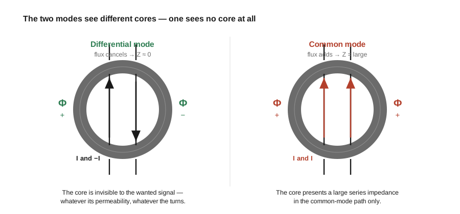
The fix follows directly from §2’s observation that the two modes are independent: build a device that is transparent to the differential mode and opaque to the common mode. A ferrite core does this, and the reason is a flux argument that takes one paragraph.

Wind several turns of the feedline through a ferrite toroid. Consider the differential mode first: I₁ on the centre conductor and I₂ = −I₁ on the inner shield surface pass through the core together, in the same turns, in opposite directions. Their magnetic fields are equal and opposite, so the net flux they drive in the core is zero. A core that carries no flux stores no energy and presents no impedance. The core is invisible to the wanted signal — the differential mode passes with Z ≈ 0, and this is true regardless of how permeable the core is or how many turns are used.

Now the common mode: I₃ on the outer shield surface passes through those same turns with nothing to cancel it. Its flux adds turn by turn. The wound assembly is, to the common mode, simply an inductor with a high-permeability core, and it presents a large series impedance in the common-mode path.

Two things about this deserve emphasis because they are the source of persistent confusion.

A current balun is a choke, not a transformer. In the 1:1 case there is no impedance transformation happening at all, and calling it a “1:1 transformer” invites the question of what a 1:1 transformer could possibly be for. The answer is that it is not transforming; it is choking. The device’s figure of merit is not a turns ratio but a common-mode impedance, usually written Z_cm, measured in ohms, and strongly frequency-dependent. Vol 2 shows how the same transmission-line structure, with its ends connected differently, becomes an impedance transformer as well — but the 1:1 case is pure choke.

The core’s properties matter only to the common mode. This is a useful diagnostic. If a “balun” degrades the differential path — if it raises SWR, or gets hot with a matched load, or shows insertion loss — then something other than the flux-cancellation mechanism is going on: a winding whose characteristic impedance is wrong, a core in saturation, or a topology that is not actually a current balun. A correctly built current balun with a matched load is close to a piece of wire in the differential path. Vol 3 develops the loss mechanism properly; Vol 5 uses this as a build check.

1.6 High impedance is not enough — resistive versus reactive

Here is where the received wisdom fails, and it fails in a direction that surprises people: a choke with several hundred ohms of impedance can make the common-mode current larger than no choke at all.

The reason is already visible in §3. The common-mode path is not resistive; Hunt’s worked example put it at about 28 − j200 Ω. Impedances in series add. If the choke you insert is inductive — a reactance of +j200 Ω, say, which is a perfectly ordinary thing for a wound ferrite choke to be at some frequency — then it does not add to the path impedance. It cancels part of it:

    without choke:   Z_cm  =  28 − j200 Ω        |Z| ≈ 202 Ω
    with +j200 Ω:    Z_cm  =  28 − j200 + j200
                           =  28 + j0 Ω          |Z| ≈  28 Ω

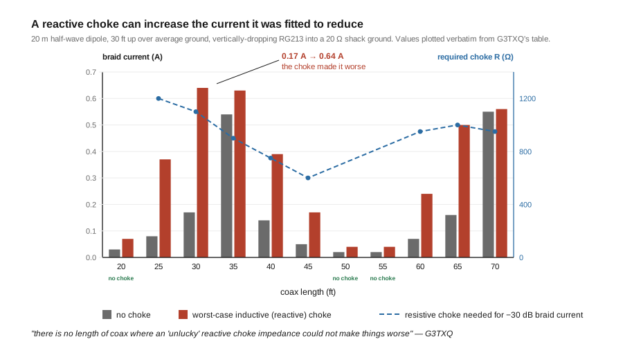
The path impedance has fallen by a factor of seven, and the common-mode current rises accordingly. Hunt’s EZNEC model gives the numbers: the braid current goes from 0.17 A with no choke to 0.64 A with the reactive choke installed — “that’s a majority of the current flowing at the feedpoint!”

That is not a contrived worst case in the sense of being unlikely. Hunt is explicit about the width of the trap: “any choke reactance between 0 and +j400 will reduce the CM path impedance — and therefore increase the braid current — to some degree.” A wound choke sweeps through that entire range as frequency changes.

Nor is it escapable by choosing a lucky feedline length. He tabulates the model across coax lengths from 20 ft to 70 ft and concludes: “there is no length of coax where an ‘unlucky’ reactive choke impedance could not make things worse!”

The design rule that follows is Hunt’s own, and it is the sentence to carry out of this volume: “Aim to choose a choke which has a high impedance and is Resistive over the frequency range of interest.” A resistive choking impedance cannot cancel anything. It adds to the path impedance monotonically, whatever the path’s reactance happens to be, so it is safe at every frequency and every feedline length. His conclusion is unambiguous: “a high value Resistive choke is the safe option for all scenarios.”

This is why his published choke charts mark, separately from the impedance magnitude, the frequency range over which each choke’s impedance is predominantly resistive — his criterion is Rs > |Xs|. Two chokes with identical impedance magnitude at 7 MHz are not equally good if one is 1 kΩ of resistance and the other is 1 kΩ of reactance. The material that determines which you get is the subject of Vol 3; the short version is that this is the single strongest argument for choosing core material by measured Z_cm curves rather than by permeability.

One important qualification, and it is Hunt’s, not a hedge added here — the point is not that reactance is worthless. He notes: “when the reactive component of the CM path impedance exceeds +/-1000 Ω there is also likely to be a large resistive component; this means that reactive chokes may still contribute useful choking impedance provided their reactance is several kΩ.” A choke with 5 kΩ of reactance is not going to be cancelled into insignificance by a path reactance of a couple of hundred ohms. The trap is specifically the moderate reactive choke — a few hundred ohms, comparable to the path’s own reactance. Which is, unhelpfully, exactly what an under-turned ferrite choke provides at the low end of its range.

Note also what the air-cored “ugly balun” does under this criterion. Hunt’s chart shows no resistive-range markers at all for the air-cored chokes, because “their impedance is almost entirely Reactive apart from a very small band of frequencies around resonance.” An air-wound coil of coax is a purely reactive choke by construction. It is not a broadband solution; it is a single-frequency expedient, and away from its self-resonance it is the exact device this section warns about.

1.7 How much choking impedance is enough

With “resistive” established as the qualitative requirement, the quantitative question is how many ohms. Two answers circulate, and one of them is wrong.

The common rule of thumb sets the target at some multiple of the differential-mode load impedance — “ten times the feedpoint impedance”, or a flat “at least 1 kΩ”. Hunt’s model tests this and rejects it: “Rules-of-Thumb which equate the required choke impedance to some multiple of the differential-mode load impedance are unsound.”

The reason is structural. The common-mode current is set by a voltage divider between the choke’s impedance and the impedance of the common-mode path — and the common-mode path is a property of the installation: the feedline’s length and routing, the ground connection, the surroundings. The differential-mode load impedance does not appear in that divider. The two quantities are unrelated, so a rule relating them cannot be right except by coincidence.

The defensible answer comes from asking what suppression you want and computing the resistance that delivers it. Hunt does exactly this, tabulating for each coax length the choke resistance required to hold the braid current 30 dB below the dipole current (that is, 0.03 A for the 1 A feedpoint current in his model):

Table 1 — The defensible answer comes from asking what suppression you want and computing the resistance that delivers it. Hunt does exactly this, tabulating for each coax length the choke resistance required to hold the braid current 30 dB below the dipole current (that is, 0.03 A for the 1 A feedpoint current in his model)

Coax length (ft)	Braid current, no choke (A)	Braid current, worst-case inductive choke (A)	Choke resistance for −30 dB braid current
20	0.03	0.07	No choke needed
25	0.08	0.37	1200 Ω
30	0.17	0.64	1100 Ω
35	0.54	0.63	900 Ω
40	0.14	0.39	750 Ω
45	0.05	0.17	600 Ω
50	0.02	0.04	No choke needed
55	0.02	0.04	No choke needed
60	0.07	0.24	950 Ω
65	0.16	0.50	1000 Ω
70	0.55	0.56	950 Ω

Reproduced verbatim from the table in Hunt’s “Common-mode chokes”; the model is the 20 m dipole described in §3. No rows have been added, interpolated or rounded.

Three things to take from this table, and one caution.

The required resistance is roughly 600–1200 Ω across the lengths that need a choke. That is where the widely-quoted “aim for a kilohm or more” gets its number, and as a target for this class of installation it is sound — it is the derivation via load impedance that is unsound, not the figure.

The requirement varies by more than 2:1 with feedline length alone, over a range of lengths any real installation might use. It is not a property of the antenna.

Four of the twelve lengths need no choke at all — and they are interleaved with lengths that need 1200 Ω. There is no smooth trend to extrapolate along; 50 ft and 55 ft need nothing while 65 ft needs 1000 Ω. Hunt gives the mechanism: “When the coax is close to a quarter-wave long the CM path is high-impedance and relatively little current flows along the braid whether we include a choke or not; when it is close to a half-wavelength long substantial current flows if we don’t include a choke.” An operator cannot know which case they are in without measuring, which is the practical argument for simply always fitting a good resistive choke.

The caution: this is one model of one antenna at one height with one ground. The numbers are the right order of magnitude and the right shape, and they are quoted here because they are published, reproducible and specific — but a 1 kΩ resistive target is a well-founded default, not a universal constant. A multiband antenna is harder; Hunt notes that “with a multiband antenna — in fact the potential for a Reactive choke exacerbating the situation on at least one of the bands increases.” The honest summary is: aim for at least ~1 kΩ, resistive, across every band you use, and understand that this target is derived from modelling of a representative case rather than measured on yours.

1.8 Balance and impedance are two different problems

Everything so far has been about balance. The other half of the family exists for a different reason, and keeping the two apart is the single most useful piece of vocabulary hygiene in this subject.

• A BALUN (BALanced-to-UNbalanced) connects an unbalanced line to a balanced load. Its defining job is the one developed in §§2–7: keeping current off the outside of the shield. It may also transform impedance.
• An UNUN (UNbalanced-to-UNbalanced) has an unbalanced, single-ended connection on both sides. Its defining job is impedance transformation. It does not address balance, because with both sides single-ended there is no balance to enforce.

The pairing with antenna types follows from the antenna’s own symmetry:

• A centre-fed dipole, folded dipole, off-centre-fed dipole, doublet or Yagi driven element is a balanced structure — two symmetric halves driven against each other. It needs a balun.
• An end-fed wire, random wire, EFHW, or vertical against radials is not balanced. It is a single conductor worked against a ground or counterpoise. It needs an unun for the impedance, and — this is the part that trips people — it still has a common-mode problem, because the coax shield can perfectly well act as the counterpoise whether you intended it to or not. An end-fed antenna typically wants an unun for the ratio and a separate choke for the balance. Vol 4 takes this up in detail; it is why a well-designed EFHW transformer assembly often contains two cores doing two different jobs.

The mirror-image confusions are worth naming explicitly, because both are common and both cost money:

“A common-mode choke and a balun do the same thing.” A 1:1 current balun and a common-mode choke are essentially the same device — that much is fair. But a 4:1 or 49:1 device transforms impedance as well, and a bead-string choke transforms nothing. Buying a 49:1 unun to cure RF in the shack does not work; neither does buying a bead choke to feed a folded dipole.

“If the SWR is 1:1 the balun is working.” SWR is a differential-mode measurement. §5 showed that a correct current balun is nearly invisible to the differential mode — which means a good balun, a bad balun, and a shorting link all read about the same on an SWR meter with a matched load. SWR tells you about the impedance job and nothing whatsoever about the balance job. This is exactly why Vol 5 replaces the seed material’s SWR-with-a-dummy-load procedure with a series-through fixture that measures Z_cm directly: measuring the wrong quantity carefully is not verification.

1.9 The feedpoint catalogue — what sets the ratio

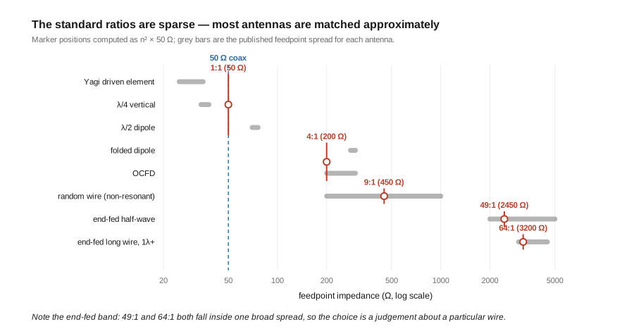
The transformation ratio is not a free choice. It comes from the antenna’s feedpoint impedance, and the operator’s job is to pick the standard ratio nearest to it. For a transformer, impedance ratio is the square of the turns ratio:

    Z_ant / Z_line  =  n²          n = turns ratio (secondary : primary)

    so    n  =  √( Z_ant / 50 )    for 50 Ω coax

Which gives the ladder of standard ratios and the impedance each one is built to serve:

Table 2 — Which gives the ladder of standard ratios and the impedance each one is built to serve

Antenna	Feedpoint Z	Ratio	Turns ratio n	Device
Yagi driven element (closely-coupled design)	25–35 Ω	1:1	1	1:1 current balun (matching done in the array)
λ/4 vertical over an extensive radial field	≈ 36 Ω	1:1	1	1:1 choke (no transformation wanted)
Centre-fed λ/2 dipole, resonant	≈ 73 Ω	1:1	1	1:1 current balun
Folded dipole	≈ 4 × 73 ≈ 290 Ω	4:1	2	4:1 current balun
Off-centre-fed dipole (OCFD)	≈ 200–300 Ω	4:1	2	4:1 current balun
Random wire, non-resonant	≈ 200–1000 Ω, band-dependent	9:1	3	9:1 unun (+ tuner)
End-fed half-wave, at the end	≈ 2450 Ω nominal	49:1	7	49:1 unun
End-fed long wire, 1λ and up	≈ 3000–4500 Ω	64:1	8	64:1 unun

Three observations that matter more than the table itself.

The 4:1 for a folded dipole is not a coincidence, it is the same factor twice. A folded dipole steps its feedpoint impedance up by exactly 4 because the current divides between two conductors — the step-up is 4 × 73 ≈ 290 Ω, and a 4:1 balun steps it back down to ≈ 73 Ω, which is then fed by 50 Ω coax at the same benign 1.46:1 mismatch a plain dipole presents. The folded dipole and its balun are designed together. See Single-Band Dipoles Vol 4 for the step-up derivation.

The 2450 Ω figure for an EFHW is the ratio’s implication, not a measurement. This is worth being precise about, because the seed material for this dive stated it the other way round and the circularity is easy to miss. 49 × 50 = 2450, so a 49:1 transformer is by construction matched to 2450 Ω. The actual endpoint impedance of a real half-wave wire is not a constant — it depends on height above ground, on frequency, and on the wire’s surroundings, and published measurements spread over a range from roughly two to five kilohms. The 49:1 ratio became standard because it lands in the middle of that spread and leaves a mismatch the rig can live with, not because 2450 Ω is a physical constant of half-wave wires. Vol 4 treats the consequences, which include why the same 49:1 transformer gives noticeably different SWR on different bands of the same wire.

The spread inside a row is often larger than the gap between rows. A random wire is quoted at 200–1000 Ω; a 9:1 unun serves 450 Ω exactly and everything else approximately. This is not a defect in the table — it is why a random-wire installation includes a tuner and an EFHW does not. A ratio is a coarse transformation that gets the impedance into a range something else can finish; expecting a fixed-ratio transformer to deliver 1.1:1 across five bands is expecting the wrong thing from it.

1.10 Where this volume hands off

This volume established the problem and the mechanism. Four things were deliberately deferred, each to the volume that can do it properly:

• How the structure is actually built — Guanella’s series-parallel transmission lines, Ruthroff’s bootstrap, why the voltage balun degrades at high ratios, and the transmission-line-transformer condition that the wound line’s characteristic impedance should be the geometric mean of the impedances it works between: Vol 2.
• Which core material puts resistive choking impedance where you need it — the §6 criterion turned into a material choice, with the complex permeability that explains why a ferrite choke is a resistor at HF and the measured Z_cm curves that settle the mix-31-versus-mix-43 question: Vol 3.
• The ratios in practice — 1:1, 4:1, 9:1, 49:1 and 64:1 against the antennas that need them, the corrected EFHW autotransformer arithmetic, and the compensation capacitor: Vol 4.
• Building and verifying one — BOMs and step-by-step winding for the canonical five, the series-through fixture that measures common-mode impedance rather than SWR, and a dated commercial survey: Vol 5.

Outward, the antenna dives that end at a feedpoint this dive serves: Single-Band Dipoles for the 73 Ω feedpoint and its 1:1 choke, Multi-Band Dipoles for the OCFD and folded cases, Random Wire & End-Fed for the 9:1 and 49:1 cases, Fixed Vertical Monopoles for the radial-field ground system that sets a vertical’s feedpoint, and Yagi-Uda for the matching topologies that live inside the array rather than at the feedpoint. Measurement technique is NanoVNA.

1.11 Resources

• Hunt, S. E. (G3TXQ), “Common-mode chokes.” The measurements and the EZNEC model this volume’s §§3, 6 and 7 draw on, including the coax-length table reproduced in §7, the 28 − j200 Ω common-mode path example, the resistive-versus-reactive criterion (Rs > |Xs|), and the published choke-impedance charts for #31, #43, #52 and #61 240-size toroids at 5, 9, 12 and 17 turns on single, 2-stacked and 4-stacked cores. Chart last updated 15 May 2012; page last updated 6 December 2017. © 2007/18 S E Hunt G3TXQ.
• Sevick, J. (W2FMI), Transmission Line Transformers. The canonical text on the transmission-line-transformer family; the reference for Vol 2’s topology derivations.
• Maxwell, W. (W2DU), Reflections. The origin of the bead-string choke balun and the clearest treatment of why a feedline’s behaviour is not what a naive SWR reading suggests.
• Fair-Rite material data sheets. Published initial permeability, complex-permeability curves and stated application frequency ranges per mix — the primary source for Vol 3.
• ARRL Antenna Book, current edition — the standard reference for the feedpoint impedances catalogued in §9.