The Ratios in Practice — 1:1, 4:1, 9:1, 49:1 and 64:1

---

4.1 About this volume

Vol 1 said what the two jobs are, Vol 2 how the structures work, Vol 3 what the core has to be. This volume is the catalogue: the five ratios an operator actually buys or winds, what each is for, and how to choose between them.

It is also where the largest single error in the seed material for this dive gets corrected. The EFHW transformer — the most-built matching device in amateur radio over the last decade, and the load-bearing component in every end-fed installation this hub describes — was written up with its turns arithmetic wrong, and with an invented physical mechanism papering over the mistake. §7 does that properly.

The other thing this volume tries to do is displace a habit. The ratios are usually presented as a lookup table: this antenna, that ratio. That works until the antenna is not one of the listed ones, or the listed impedance is not what yours measures. The better framing is that a fixed-ratio transformer is a coarse step whose job is to land the impedance somewhere a rig or a tuner can finish, and the question is always how much error the step leaves. §§2–3 set that up numerically before the catalogue starts.

4.2 Choosing a ratio from a measured feedpoint

The rule from Vol 1 §9 is that impedance ratio is the square of the turns ratio, so for 50 Ω coax:

    n  =  √( Z_ant / 50 )

and the available ratios are the perfect squares, for the topological reason Vol 2 §8 derived. So the procedure is:

1. Measure the feedpoint. Not look it up — measure it, at the frequencies you intend to use, with the antenna installed at its real height over your real ground. NanoVNA Vol 4 covers the measurement. Published feedpoint impedances are starting points; a wire’s surroundings move them substantially.
2. Compute the ideal ratio as Z_ant / 50.
3. Take the nearest standard ratio, and compute what mismatch that leaves.
4. Decide whether the remaining mismatch needs a tuner.

Step 3 is where the interesting part lives, because the standard ratios are sparse — and, computing rather than assuming, the sparseness costs less than one would guess almost everywhere, and more than one would guess in one narrow place.

A worked pair, both computed:

• 700 Ω. Ideal ratio 14:1. The nearest commonly-sold part is the 9:1, which leaves 700/9 = 77.8 Ω — an SWR of 1.56:1. No tuner needed. This is not a gap, despite falling between two standard ratios.
• 1125 Ω. Ideal ratio 22.5:1. The best commonly-sold part is the 49:1, leaving 1125/49 = 23 Ω — an SWR of 2.18:1. That is the worst the family does anywhere in its range, and it is where a 16:1 or 25:1 would land at 1.1:1 if either were a normal amateur part.

The arithmetic for step 3, given a chosen ratio r:

    Z′  =  Z_ant / r                  the impedance the rig sees
    SWR =  max( Z′/50 , 50/Z′ )       for a purely resistive Z′

That second line assumes the feedpoint is resistive, which at resonance it approximately is. Off resonance there is reactance too and the SWR is worse than this formula gives — so treat it as a floor, not a prediction.

4.3 How much each ratio actually covers

Plotting the SWR of §2 against the actual feedpoint impedance, for each standard ratio, shows the family’s coverage and its gaps at a glance.

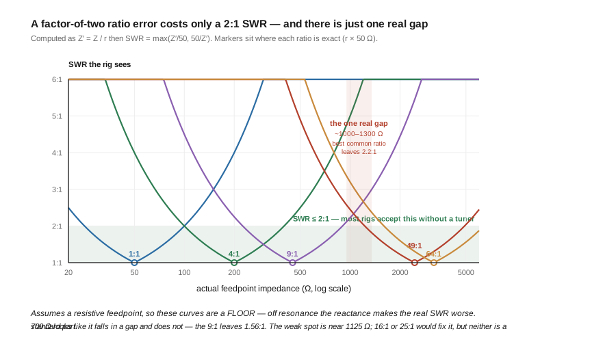
The design consequence, and it is worth stating plainly because it cuts against how the ratios are usually taught: a ratio error of a factor of two costs only a 2:1 SWR. SWR is a forgiving function of a transformation error. That is why a single 49:1 transformer serves a wire whose real endpoint impedance wanders over a couple of kilohms across the bands, and why arguing about whether a particular wire “really” wants 49:1 or 64:1 is usually arguing about a few tenths of an SWR point.

What is not forgiving is the Vol 1 §6 common-mode problem, which no ratio addresses at all. An operator who spends effort optimising the ratio and none on the choke has optimised the forgiving variable and ignored the unforgiving one.

4.4 The 1:1 — and when a 1:1 is not a transformer at all

The 1:1 is the most-installed device in the family and the one most often misunderstood, because in its usual form it performs no transformation whatsoever.

A resonant centre-fed dipole is about 73 Ω. Fed with 50 Ω coax that is a 1.46:1 SWR, which every rig accepts. There is nothing to transform. The device at that feedpoint is there for balance — it is the common-mode choke of Vol 1, and calling it a “1:1 balun” invites the reasonable question of what a 1:1 transformer could be for.

So:

• A 1:1 current balun / choke — the Guanella 1:1 of Vol 2 §3. Wind the feed coax through a core. Z₀ = 50 Ω is automatically right because the coax is the line (Vol 2 §7). This belongs at every coax-fed feedpoint in the hub.
• A 1:1 voltage balun — a real transformer, galvanically isolating, occasionally wanted where a genuine DC break or a defined ground reference matters. Rare at an antenna feedpoint, and per Vol 2 §5 the wrong choice there.

The practical error to avoid is buying a 1:1 device on impedance grounds. A Yagi driven element at 25 Ω and a quarter-wave vertical at 36 Ω are both fed through 1:1 chokes, not because 1:1 matches them — it does not — but because their mismatch is tolerable and the matching, where any is needed, is done inside the array or with a matching section. The choke is doing the balance job regardless.

4.5 The 4:1 — off-centre-fed and folded dipoles

The 4:1 transforms 200 Ω to 50 Ω, and two antennas want it for genuinely different reasons.

The folded dipole steps its own feedpoint up by exactly 4, to about 4 × 73 = 290 Ω, because the current divides between two conductors. A 4:1 step-down returns it to ≈ 73 Ω, and the rig then sees the same benign 1.46:1 a plain dipole gives. The antenna and its transformer were designed together; see Single-Band Dipoles Vol 4 for the step-up derivation.

The off-centre-fed dipole presents 200–300 Ω at its design frequency because the feedpoint has been moved off the current maximum deliberately, to make one wire resonate usefully on several bands. Here the 4:1 is doing a real impedance job. Multi-Band Dipoles Vol 1 covers the OCFD family.

Both are balanced antennas, so both want a current 4:1 — the Guanella of Vol 2 §3, two lines with their inputs paralleled and outputs in series. And per Vol 2 §7 each of those two lines wants Z₀ = √(50 × 200) = 100 Ω, which is why a 4:1 Guanella is wound with a spaced bifilar pair rather than with 50 Ω coax. Winding one with coax to hand puts a mid-band dip in it for no reason.

A Ruthroff (voltage) 4:1 will work into a symmetric low-impedance load and is common in tuners. At an asymmetric wire feedpoint it hands the asymmetry back to the coax shield as common-mode current, which is Vol 2 §2’s whole argument.

4.6 The 9:1 — a coarse step with a tuner behind it

The 9:1 transforms 450 Ω to 50 Ω, and it exists for antennas that have no single feedpoint impedance to match.

A random wire — a non-resonant length, fed at one end against a counterpoise — presents anything from a couple of hundred ohms to a kilohm or more depending on band, and its reactance is large and swings through zero at unpredictable places. There is no ratio that matches it. The 9:1’s job is to drag that whole wandering range down into a span a tuner can finish, and 450 Ω sits near the geometric middle of what a random wire typically does. See Random Wire & End-Fed Antennas.

Two things follow that are frequently missed:

A 9:1 unun without a tuner is an incomplete installation. The device is not a match; it is a range-shifter. Selling or describing a 9:1 as a way to “make a random wire work on all bands” without mentioning the tuner overstates it.

A 9:1 is an unun, so it does not address balance at all — both sides are single-ended. The end-fed wire works against something, and if you have not given it a counterpoise the coax shield will volunteer. §10 takes this up.

Construction: as a Guanella it is three lines at Z₀ = √(50 × 450) = 150 Ω (Vol 2 §8); as a trifilar autotransformer it is one winding of three twisted wires with the taps connected in series. The autotransformer form is much the more common, and since there is no balance to preserve, that trade is sound (Vol 2 §10).

4.7 The 49:1 EFHW transformer, and the arithmetic corrected

This is the most-built matching device in modern amateur radio and the section where the seed material for this dive went wrong. The correction matters because every end-fed installation in the hub rests on it.

4.7.1 What the seed said, and why it is wrong

The seed described the standard winding as “a 2-turn primary + 14-turn secondary autotransformer”, then reasoned:

“Turns ratio: 2+14 = 16 total turns, with the antenna wire connected after 16 turns and the coax driving the first 2 turns. Impedance ratio: (16/2)² = 64? No — the 49:1 ratio comes from accounting for the magnetic coupling and the autotransformer’s effective turns ratio. The full math is in Sevick, but the empirical fact is: this winding gives 49:1 transformation.”

Two things went wrong there, and the second is worse than the first.

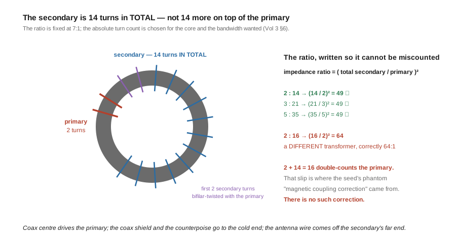
The arithmetic error. In the conventional notation, a 2 : 14 transformer has a primary of 2 turns and a secondary of 14 turns in total — not 14 additional turns on top of the primary. The turns ratio is therefore:

    n  =  14 / 2  =  7          →      impedance ratio  n²  =  49

Adding the primary to the secondary double-counts it. The seed’s “2 + 14 = 16” is that double-count, and (16/2)² = 64 is the arithmetic consequence of it.

The invented mechanism. Having got 64 where it expected 49, the seed attributed the discrepancy to “magnetic coupling and the autotransformer’s effective turns ratio”, cited Sevick without a page, and closed with “the empirical fact is”. There is no such correction. The ratio is (N_sec / N_pri)², exactly, and the discrepancy was a counting mistake. Inventing a physical effect to reconcile an arithmetic slip is the more serious failure of the two, because it teaches the reader that the simple relation cannot be trusted — when it can.

4.7.2 What the standard winding actually is

The ratio is what is fixed; the absolute turn counts are not. Published designs use 2 : 14, 3 : 21 and 5 : 35 — all of which are 7:1 and therefore 49:1. The absolute count is chosen for the core and the bandwidth wanted, exactly the Vol 3 §6 trade: more turns pushes the useful region down in frequency.

So the rule to carry away is about the ratio, and it is worth writing in a form that cannot be miscounted:

    impedance ratio  =  ( total secondary turns  /  primary turns )²

    2 : 14   →  (14/2)²  =  49        3 : 21  →  (21/3)²  =  49
    5 : 35   →  (35/5)²  =  49        2 : 16  →  (16/2)²  =  64

⚠ Note the last line, because it is where the confusion comes from: 2 : 16 genuinely is 64:1. The seed’s (16/2)² = 64 is not a wrong calculation — it is a correct calculation of a different transformer. The error was believing 2:14 and 2:16 were the same winding.

4.7.3 How the primary is coupled

The seed also filed 49:1 and 64:1 ununs as plain single-wire autotransformers, which is incomplete. Both constructions are in use:

• The autotransformer proper. One continuous winding with the coax driving the first few turns and the antenna taken from the end. Simple, and the form Vol 2 §10 explains is chosen at this ratio because a seven-line Guanella at Z₀ = 350 Ω is impractical.
• The primary bifilar-coupled to the secondary’s first turns — the more common form in published designs. The primary’s turns are twisted together with the first turns of the secondary rather than merely being the first turns of it. The purpose is coupling: Ruthroff’s condition that “it is important that the coupling be high at all frequencies or the transformer action fails” (Vol 2 §9) is exactly what the twist improves, and a tightly-coupled primary extends the transformer’s high-frequency end.

Some designs also put a crossover in the secondary to manage the winding’s self-capacitance. These are refinements on the same 7:1 ratio, not different ratios.

4.7.4 And a caution about 2450 Ω

49 × 50 = 2450, so a 49:1 transformer is by construction matched to 2450 Ω. Vol 1 §9 made the point that this is the ratio’s implication and not a measured property of half-wave wires, whose real endpoint impedance spreads over roughly two to five kilohms with height, frequency and surroundings. §3’s coverage plot is the reason that is tolerable: across that whole spread the 49:1 leaves an SWR most rigs will accept, which is why the ratio became standard.

It also explains a common observation that otherwise looks like a fault: the same 49:1 transformer gives noticeably different SWR on different bands of the same wire. That is the wire’s endpoint impedance changing, not the transformer misbehaving.

4.8 The compensation capacitor

Most EFHW transformers include a small capacitor, typically 100–150 pF, and the seed’s account of what it does is roughly right while being vague about where it goes and why.

The mechanism: the primary is a small number of turns on a ferrite core, so it has inductance, and that inductance is a series reactance rising with frequency. At the top of HF it is large enough to spoil the match. A capacitor in parallel across the primary resonates against that inductance near the upper end of the range, cancelling part of the reactance and flattening the transformation there. Without it the SWR at 28–30 MHz climbs; with it the device holds a usable match across 3.5–30 MHz.

Three practical points:

• It is a high-voltage part. It sits across the transformer at the high-impedance end of the system, where voltages at legal power are substantial. A small ceramic disc is not adequate; the standard choice is a mica or high-voltage ceramic part rated a few kV.
• Its value interacts with the turns count, since what it resonates against is the primary’s inductance. A design that changes from 2:14 to 3:21 changes the primary inductance and therefore wants a different capacitor. Copying a capacitor value across designs without copying the winding is a common way to get a worse result than omitting it.
• It is a refinement, not a requirement. A transformer without it works, with a poorer 10 m end. This is the right thing to leave out of a first build and add while watching a sweep — which is Vol 5’s procedure.

⚠ Published designs differ on exactly where the capacitor connects — across the primary, or from the input to the antenna terminal — and those are not the same circuit. This volume describes the parallel-across-the-primary case because it is the one the mechanism above explains. Follow the specific design you are building rather than transplanting a connection point.

4.9 The 64:1, and the limits of going higher

A 64:1 is 2 : 16 turns — an 8:1 turns ratio — and matches 3200 Ω. It is used for end-fed wires appreciably longer than a half-wave, where the endpoint impedance is higher.

Two reasons it is much less common than the 49:1:

§3’s coverage plot shows the two overlapping heavily. Across the impedance range where either is plausible, the SWR difference between them is small. A 49:1 already covers most of what a 64:1 would, so the extra part number earns little.

Higher ratios get harder faster. The Z₀ a Guanella would need is √(50 × 3200) = 400 Ω (Vol 2 §8), and as an autotransformer the winding gets long, which by Vol 2 §9 pulls the high-frequency end down — precisely the end an end-fed user wants. Ratios above 64:1 are rare in amateur practice for this reason: the bandwidth cost of the extra turns outruns the matching benefit.

Where a higher transformation is genuinely wanted, the usual answer is not a bigger ratio but a different topology — an L-network, or a transformer plus a tuner — because those trade the bandwidth problem for a tuning adjustment instead. Antenna Tuners covers that route.

4.10 Two devices, two jobs

This is the section that ties the volume back to Vol 1 §8, and it is the most commonly skipped step in an end-fed installation.

An unun transforms impedance. It does not suppress common-mode current — Vol 1 §5’s flux-cancellation mechanism requires a transmission-line structure with the two modes separable, and an autotransformer has no such structure. So an end-fed antenna, which is inherently unbalanced and works against a counterpoise, has both problems and only one of them solved:

• The ratio problem, solved by the 49:1 unun.
• The balance problem — the coax shield offering itself as the counterpoise — which is entirely unaddressed.

Hence the standard, correct end-fed assembly is two devices:

    antenna wire ── [ 49:1 unun ] ── short coax tail ── [ 1:1 current choke ] ── feedline
                          │
                    counterpoise

The choke goes on the coax side of the unun, and the reason is worth understanding rather than memorising: its job is to stop current flowing on the outer surface of the feedline shield, so it has to be in that path. Placing it on the antenna side would put it in series with the high-impedance end, where it does nothing useful and sees large voltages.

This is why a well-made commercial EFHW assembly often contains two cores, and why the cheap ones that contain a single core are solving half the problem. It is also why Vol 3 §7’s mix guidance matters twice over, for two devices with different requirements: the unun’s core is chosen for transformer action and power, the choke’s for a resistive Z_cm on the bands in use.

4.11 Saturation belongs here, not to the choke

Vol 3 §8 argued that saturation is usually the wrong worry for a choke, whose limit is thermal. The high-ratio transformers in this volume are where saturation genuinely belongs, and the distinction is about what the core carries.

A 1:1 choke sees the differential mode’s flux cancel — that is the whole mechanism — so its core carries flux only from the (small) common-mode current. A 49:1 autotransformer is a real transformer: the full transmitter current flows through its primary, and that flux does not cancel. Add the lowest band, where reactance is least and flux density greatest, and full legal power, and core saturation becomes a real limit rather than a theoretical one.

The symptoms differ usefully from the thermal ones:

• Saturation appears as SWR that shifts during a transmission and returns between them, worse on the lowest band, and worse at higher power — because the flux excursion depends on voltage and frequency, not on average heating.
• Overheating appears as SWR and performance drifting over minutes and recovering slowly, roughly independent of band.

The mitigations are different too: saturation wants a larger core, more turns, or a higher-saturation mix — which is one reason mix 52’s datasheet advertises “a high saturation flux density and a high Curie temperature” (Vol 3 §5) — whereas overheating wants more surface area, stacked cores, or lower duty. Reaching for the wrong remedy is common. Vol 5’s BOMs size for the lowest band and the power actually used.

4.12 Where this volume hands off

• Building any of these, with real part numbers and step-by-step winding, plus the series-through S21 fixture that measures a choke properly and the sweep that tells you whether a transformer is right: Vol 5.
• Why the ratio is the square of the turns ratio, why the available ratios are perfect squares, and the Z₀ each Guanella line needs: Vol 2.
• Which mix, and why saturation and heating are different failures: Vol 3.
• The common-mode problem §10’s second device exists for: Vol 1.

Outward, the antennas that need each ratio: Single-Band Dipoles (1:1), Multi-Band Dipoles (4:1, OCFD), Random Wire & End-Fed Antennas (9:1 and 49:1), Transmitting Loops and Yagi-Uda Vol 3 for matching done inside the array instead. Measurement: NanoVNA Vol 4. The tuner route for what a fixed ratio cannot reach: Antenna Tuners.

4.13 Resources

• Sevick, J. (W2FMI), Understanding, Building, and Using Baluns and Ununs: Theory and Practical Designs for the Experimenter. The standard working-through of each ratio in the family. ⚠ Cited by the seed material as authority for a “magnetic coupling correction” to the 49:1 turns ratio, without a page reference; §7.1 shows no such correction is needed, and a citation used to support an arithmetic slip is worse than no citation.
• Ruthroff, C. L., “Some Broad-Band Transformers”, Proc. IRE, August 1959, pp. 1337–1342. The coupling condition §7.3 invokes.
• Published EFHW transformer designs using 2:14, 3:21 and 5:35 windings — the evidence in §7.2 that the ratio is fixed at 7:1 while the absolute turn count is a core-and-bandwidth choice. ⚠ These vary in where the compensation capacitor connects; §8 flags that they are not interchangeable.
• Hunt, S. E. (G3TXQ), “Common-mode chokes.” The basis for the second device in §10.
• Fair-Rite material data sheets. Mix 52’s saturation-flux and Curie-temperature claims quoted in §11.