Why a Small Loop Radiates At All

---

1.1 About this volume

The small transmitting loop is the strangest antenna in this hub, and the one about which the most confident wrong things are said. It is a metre of copper tubing bent into a circle with a capacitor across the gap. It has no ground system, no radials, no resonant length to cut, and it does not care much what is near it. It fits on a balcony. And it will work HF from inside an apartment, which almost nothing else will.

It is also the antenna where every important number is computable — because its defining property, a very high Q, comes from a ratio of two resistances that can both be written down. That makes this dive unusually checkable, and the checking found a good deal.

This volume is about the radiator: why a loop that is a small fraction of a wavelength across radiates at all, what that costs, and where the standard model stops being true. Vol 2 takes the consequences of the high Q — bandwidth, the tuning capacitor and the voltage across it. Vol 3 covers the completely different family of full-wave loops. Vol 4 is pattern, siting and operating. Vol 5 builds one and surveys what to buy.

Three of this volume’s conclusions correct the previous edition, and one of them corrects it in a direction worth stating carefully.

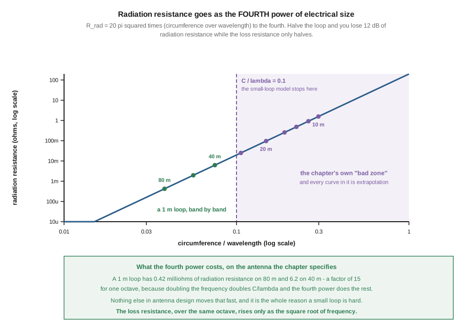
The first is the fourth-power law and what it implies. A small loop’s radiation resistance goes as (C/λ)⁴. §3 works out what that means for the antenna the previous edition specifies: a 1 m loop has 0.42 milliohms of radiation resistance on 80 m. Not ohms — milliohms. Everything difficult about this antenna follows from that one number.

The second is that the efficiency claim is wrong by more than four times, and the honest correction is not “magloops don’t work”. The previous edition states that “a 1 m copper-tube magloop is 80% efficient on 40 m.” Computed for exactly that antenna, it is 18.5 %, and on 80 m it is 2.1 %. But 18.5 % is −7.3 dB, which is a real antenna that makes real contacts, and §5 shows the more useful version of the correction: 80 % is not reachable by a small loop at all, with any conductor, because getting there means leaving the small-loop regime entirely. A builder who expects 80 % on 40 m will conclude that a correctly-built loop is faulty.

The third is that the previous edition’s own tables run three times past the boundary where its own physics applies — and into a region that same chapter tells the reader to avoid. §2 draws the boundary and every figure in this dive marks it.

1.2 Three regimes, and the boundary that matters

A loop’s behaviour is set almost entirely by its circumference relative to wavelength, and there are three genuinely distinct regimes.

Below about C/λ = 0.1 the current is nearly uniform all the way round the loop. That uniformity is what makes the loop a magnetic dipole — its far field is set by the magnetic moment I·A, not by any current distribution along a length. This is the small loop, and it is this volume’s subject.

Around C/λ = 1 the loop is a full wavelength of conductor and carries a standing wave with current maxima and minima, exactly like a folded dipole bent into a closed shape. That is a resonant current-element antenna with dipole-class bandwidth and dipole-class feedpoint impedance, and it is Vol 3’s subject. The two families share a name and essentially nothing else.

Between them is the region the previous edition calls the “bad zone” — too large for uniform current, too small to be resonant. Its own summary is right: “practical loop antennas avoid this zone.”

1.2.1 The boundary is not decorative

That C/λ ≲ 0.1 figure is the validity limit of every formula in this volume. Past it the uniform-current assumption fails, the radiation resistance departs from the fourth-power law, and numbers computed from the small-loop model become extrapolation rather than prediction.

This matters here because the previous edition’s tables run to C/λ = 0.30. Its 1 m loop, tabulated across nine bands:

Table 1 — This matters here because the previous edition's tables run to C/λ = 0.30. Its 1 m loop, tabulated across nine bands

band	80 m	60 m	40 m	30 m	20 m	17 m	15 m	12 m	10 m
C/λ	0.038	0.056	0.075	0.106	0.149	0.190	0.222	0.261	0.299

Only 80, 60 and 40 metres are properly inside the small-loop regime. Thirty metres is at the boundary, and 17 through 10 metres are squarely inside the bad zone the same chapter says to avoid. A 1 m loop on 10 m is not a magnetic loop in any useful sense.

That is not a reason to throw the tables away — it is a reason to mark them. Every figure in this dive greys out the region past C/λ = 0.1, and where a number falls beyond it, this dive says so rather than quoting it as a result.

⚠ One small thing, since it is the kind of slip that signals hurried work elsewhere: the previous edition’s table is headed “Three loop-size regimes” and has four rows.

1.3 The fourth power

For a loop small enough that the current is uniform, the radiation resistance is

R_rad = 20π² · (C/λ)⁴

where C is the circumference. Equivalently R_rad = 31171·(A/λ²)² for loop area A — the same statement, since area and circumference are locked together for a circle.

That fourth power is the single most consequential fact about this antenna, and the lead figure plots it. Read the exponent literally: halve the loop and you lose 12 dB of radiation resistance. Nothing else in antenna design punishes size that hard. A half-wave dipole cut to half its length loses a couple of dB; a loop halved loses a factor of sixteen.

Worked for the antenna the previous edition specifies — a 1 m diameter loop:

Table 2 — Worked for the antenna the previous edition specifies — a 1 m diameter loop

band	C/λ	R_rad
80 m	0.038	0.42 mΩ
60 m	0.056	1.96 mΩ
40 m	0.075	6.22 mΩ
30 m	0.106	25.0 mΩ

Read the first row again. Four hundred and twenty microhms. That is comparable to a short length of the tubing the loop is made from, and it is the entire resistance through which this antenna converts current into radiation on 80 metres.

Across a single octave, from 80 m to 40 m, R_rad rises by a factor of fifteen — because doubling the frequency doubles C/λ and the fourth power does the rest. That is the mechanism behind everything else in this dive: the loop is a completely different antenna on each band, far more so than any dipole or vertical, and quoting a single figure for “a magnetic loop” is close to meaningless without saying which band.

Note also what does not appear in the formula: the conductor. Radiation resistance depends on electrical size and nothing else. Fat tubing does not raise it. That is why §4’s other resistance is the one you can do something about.

1.4 The other resistance, and where they cross

Against that radiation resistance sits the loss resistance of the conductor. At HF the current flows in a skin a few tens of microns deep, so the loop’s resistance is its surface resistance times the ratio of its perimeter to the conductor’s circumference:

R_loss = (r/a)·R_s, with R_s = ρ/δ and δ = √(ρ/πfµ₀)

for loop radius r and conductor radius a. The important property is the exponent: R_loss rises only as the square root of frequency, because the skin depth shrinks as 1/√f.

So the two resistances race, and they race at wildly different speeds — one as f⁴, the other as f^0.5. The efficiency is simply

η = R_rad / (R_rad + R_loss)

and the whole of a small loop’s performance is where those two curves cross.

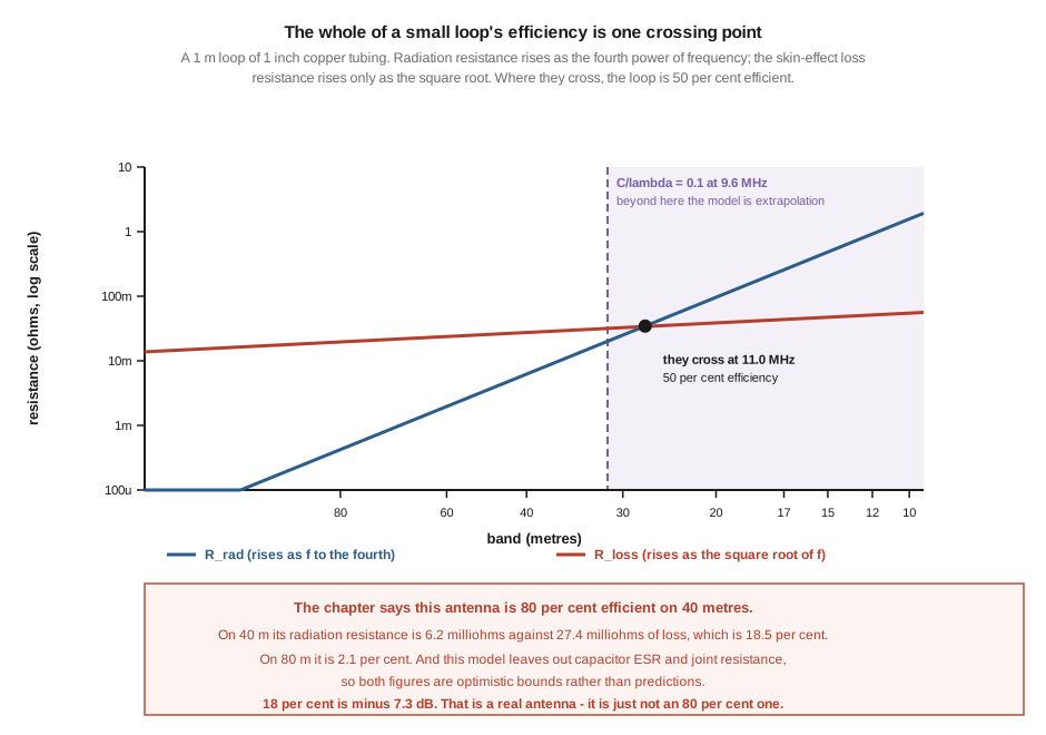
For the 1 m loop of 1″ copper the previous edition specifies, they cross at 11.0 MHz. Below that the loop is losing more than it radiates; above it, the reverse.

Table 3 — 4. The other resistance, and where they cross

band	R_rad	R_loss	efficiency
80 m	0.42 mΩ	19.6 mΩ	2.1 %
60 m	1.96 mΩ	23.8 mΩ	7.6 %
40 m	6.22 mΩ	27.4 mΩ	18.5 %
30 m	25.0 mΩ	32.6 mΩ	43.4 %

⚠ Two honesty notes belong with that table, and both push the same way. The model excludes the tuning capacitor’s own loss and the resistance of the joints where the capacitor meets the loop — and on a loop whose total resistance is twenty milliohms, a few milliohms of contact resistance is not a rounding error. Every efficiency in this dive is therefore an optimistic bound, not a prediction. And the 30 m row sits at C/λ = 0.106, just past the validity limit, so it is the least trustworthy row in the table.

1.4.1 What this does and does not say about the antenna

The previous edition’s claim is “a 1 m copper-tube magloop is 80% efficient on 40 m.” The computed figure is 18.5 %.

It would be easy, and wrong, to conclude from that that small loops are a bad idea. 18.5 % is −7.3 dB. Against a full-size dipole in the clear you are giving away a little over an S-unit; against no antenna at all — which is the actual alternative for most people who buy a magloop — you are infinitely ahead. People work DX with these antennas routinely, and the reason is that −7 dB is a real signal.

What the correction changes is expectations and diagnosis. A builder told to expect 80 % who measures a system consistent with 18 % will start looking for a fault that is not there. And a reader deciding between a magloop and, say, an end-fed wire needs the real number to make that comparison.

The useful form of the correction is not the number but the mechanism: efficiency is bought with electrical size, and only weakly with copper. Which is §5.

1.5 The ceiling a small loop cannot get past

If 18.5 % is not enough, what would it take?

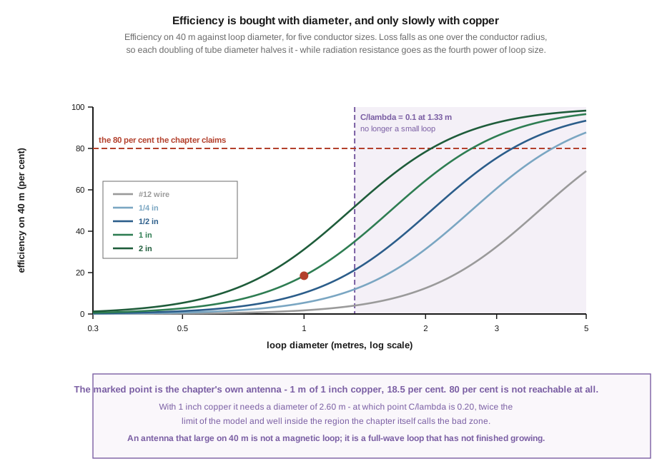
Two levers exist, and they are very unequal.

Conductor size moves loss as 1/a, so each doubling of tube diameter halves the loss resistance. On 40 m, for a 1 m loop:

Table 4 — Conductor size moves loss as 1/a, so each doubling of tube diameter halves the loss resistance. On 40 m, for a 1 m loop

conductor	efficiency on 40 m
#12 wire (2 mm)	1.8 %
¼″ tube	5.4 %
½″ tube	10.2 %
1″ tube	18.5 %
2″ tube	31.2 %
4″ tube	47.6 %

Real, and it is why every serious magloop is built from fat tubing rather than wire. But four-inch copper tube is a plumbing fantasy for most builders, and it still does not reach 80 %.

Loop diameter moves radiation resistance as the fourth power, so it is by far the stronger lever. With 1″ copper on 40 m, 80 % efficiency needs a diameter of 2.60 m.

And that is the result worth carrying:

⭐⭐ At 2.60 m on 40 m, C/λ is 0.195 — twice the small-loop limit, and inside the bad zone. The antenna that would deliver 80 % on 40 m is not a magnetic loop at all. It is a full-wave loop that has not finished growing.

1.5.1 The real ceiling

Push that further. Ask what the best possible efficiency of a genuinely small loop is — evaluate right at C/λ = 0.1, the edge of the regime.

At that boundary R_rad is fixed at 19.7 mΩ whatever the loop’s physical size, because radiation resistance depends on electrical size alone. Only the loss varies. And the loss at fixed electrical size gets worse for a bigger loop, because a bigger loop at the same C/λ means a lower frequency, a deeper skin, and more conductor:

Table 5 — At that boundary Rrad is fixed at 19.7 mΩ whatever the loop's physical size, because radiation resistance depends on electrical size alone. Only the loss varies. And the loss at fixed electrical size gets worse for a bigger loop, because a bigger loop at the same C/λ means a lower frequency, a deeper skin, and more conductor

diameter	frequency at C/λ = 0.1	best possible efficiency
0.5 m	19.1 MHz	46.8 %
1.0 m	9.5 MHz	38.4 %
2.0 m	4.8 MHz	30.6 %
3.0 m	3.2 MHz	26.4 %

A small loop of 1″ copper tops out somewhere below 50 %, and the bigger you build it the lower that ceiling gets. Not because big loops are bad — a big loop is more efficient on any given band — but because at a fixed electrical size, physical size buys you nothing and costs you conductor.

So the honest summary of the efficiency question is: a small transmitting loop is a device that trades most of your power for the ability to be small. Nothing about that is a defect, and nothing about it is hidden — it is (C/λ)⁴ doing exactly what it says. What is a defect is quoting 80 %.

1.6 Why not just use a short dipole?

Everything so far makes the small loop sound like a poor bargain, which raises the question the previous edition never asks. A magnetic loop 1 m across occupies about the same space as a 1 m short dipole. If radiation resistance is the problem, why not use the dipole?

On radiation resistance alone, the dipole wins — and it wins enormously.

Table 6 — 6. Why not just use a short dipole?

band	1 m loop	1 m short dipole	dipole ahead by
80 m	0.42 mΩ	29.3 mΩ	69×
40 m	6.22 mΩ	112 mΩ	18×
20 m	96.1 mΩ	441 mΩ	4.6×
10 m	1.57 Ω	1.78 Ω	1.1×

⚠ The bottom two rows are outside the small-loop model by §2’s own boundary — a 1 m loop is at C/λ = 0.15 on 20 m and 0.30 on 10 m — so read them as the trend rather than as figures. The 80 m and 40 m rows are inside it.

The exponents are the whole story. A short dipole’s radiation resistance goes as 20π²(l/λ)² — a square. The loop’s goes as the fourth power. Both collapse as the antenna shrinks, but the loop collapses twice as fast, so the gap widens the smaller the antenna gets electrically. On 10 m, where a 1 m structure is no longer very small, the two have almost converged.

So the loop is a worse radiator than a dipole of the same size, by a margin that is embarrassing on the low bands. And people build loops anyway. The reason is that radiation resistance is only the numerator.

1.6.1 The dipole has to find a return path

A dipole is fed against something. A full-size one is fed against its other half; a 1 m short dipole on 80 m is fed against a counterpoise, a radial field, or the ground — and that return path has resistance. Set beside 29 milliohms of radiation resistance, it does not need to be much:

Table 7 — A dipole is fed against something. A full-size one is fed against its other half; a 1 m short dipole on 80 m is fed against a counterpoise, a radial field, or the ground — and that return path has resistance. Set beside 29 milliohms of radiation resistance, it does not need to be much

the dipole’s return path	efficiency on 80 m
a good radial field, 2 Ω	1.4 %
a few radials on soil, 5 Ω	0.58 %
an indoor counterpoise, 25 Ω	0.12 %
the 1 m loop, no ground system at all	2.1 %

⭐⭐ The loop wins not by radiating better but by having nowhere else to lose the power. It is a closed circuit. There is no return path to build, no radial field to lay, and no ground resistance in series with the radiation resistance — the only loss is the conductor’s own twenty milliohms, and that is a number a builder controls with a trip to the plumbing merchant.

That is the actual case for the small transmitting loop, and it is a much better case than the one the previous edition makes. It is not an efficient antenna. It is an antenna whose inefficiency is bounded and known, in a situation where the alternatives’ inefficiency is neither.

1.6.2 And the near field is the right shape

There is a second half to it, and it is why a loop works indoors when a whip does not.

A small loop’s stored near-field energy is overwhelmingly magnetic. A short dipole’s is overwhelmingly electric. That matters because the lossy things that surround an indoor or balcony antenna — plasterboard, furniture, damp masonry, soil, people — are lossy dielectrics. They absorb from an electric near field far more readily than from a magnetic one, because they have permittivity and loss tangent but essentially unity permeability.

So the loop’s near field passes through its surroundings comparatively unbothered, while a short vertical’s couples straight into them. This is the mechanism behind the “loops tolerate poor sites” folklore, and unlike most folklore it is sound.

⚠ It is not immunity, and two limits are worth stating. Nearby conductors — aluminium window frames, wiring, gutters, a metal balcony rail — couple to a loop strongly and will both detune it and steal power; the loop’s tolerance is for dielectrics, not for metal. And the loop’s high Q means the detuning matters far more than it would on a broadband antenna, because a few kilohertz of shift is a whole bandwidth. Vol 4 takes siting; Vol 2 takes the bandwidth that makes it so sensitive.

1.7 What Chu’s limit actually forbids

The previous edition invokes the fundamental limit like this: “The Chu-Harrington limit (small antenna size constrains bandwidth × efficiency) ensures small loops can’t have wide bandwidth at high efficiency.”

The conclusion is defensible; the statement of the limit is loose in a way worth fixing, because the correct version is more useful.

Chu’s result bounds Q from below for a given electrical size. An antenna enclosed in a sphere of radius a has a minimum radiation Q that rises steeply as ka falls — roughly as 1/(ka)³ for a small antenna. That is a statement about stored energy versus radiated energy, and therefore about bandwidth. Wheeler reached the same place from the reactance side, and Harrington later extended the family to gain.

None of that is a limit on efficiency. Efficiency is a materials question — how much resistance sits beside the radiation resistance — and Chu’s derivation assumes a lossless antenna. There is no fundamental theorem preventing a small antenna from being efficient; there is a fourth-power law and a skin effect, which is a very different kind of obstacle. The portable and mobile monopole dive makes the same correction for loaded whips, where the limit is misquoted the same way.

Why does this matter practically? Because of what follows when you put loss back in.

⭐⭐ Loss lowers Q, and lower Q means wider bandwidth. So on a small loop, bandwidth and efficiency move in opposite directions — the same size loop, built worse, is broader-banded. Computed for a 1 m loop on 40 m:

Table 8 — ⭐⭐ Loss lowers Q, and lower Q means wider bandwidth. So on a small loop, bandwidth and efficiency move in opposite directions — the same size loop, built worse, is broader-banded. Computed for a 1 m loop on 40 m

conductor	efficiency	2:1-SWR bandwidth
#12 wire	1.8 %	10.1 kHz
¼″ tube	5.4 %	4.0 kHz
1″ tube	18.5 %	1.6 kHz
2″ tube	31.2 %	1.2 kHz

The worst antenna on that list has eight times the bandwidth of the best one. A small loop advertising an unusually wide bandwidth for its size is advertising its losses.

That is the loop-scale version of a result this hub keeps finding: the tuner dive showed that every number visible from the operating position improves as the system degrades, and the end-fed dive showed that transformer loss flatters SWR. Here it is again, in a third place: the easy measurement moves the wrong way. Vol 2 develops it, because bandwidth is where the small loop lives or dies.

1.8 Where this volume hands off

A small loop is a magnetic dipole, valid as such below about C/λ = 0.1, and the previous edition’s tables run three times past that into a region its own text says to avoid. Its radiation resistance goes as the fourth power of electrical size — 0.42 milliohms for a 1 m loop on 80 m — while its loss resistance rises only as the square root of frequency, and the crossing of those two curves is the whole of its efficiency. For the antenna the previous edition specifies that crossing is at 11 MHz, which puts it at 2.1 % on 80 m and 18.5 % on 40 m rather than the 80 % claimed. Fat tubing helps and diameter helps far more, but 80 % on 40 m needs a 2.6 m loop that is no longer a small loop — and a genuinely small loop of ordinary copper cannot exceed about 50 % at all. Chu’s limit does not forbid that; the fourth power and the skin effect do. What Chu forbids is bandwidth, which is Vol 2.

From here:

• Vol 2 — Q, bandwidth and the capacitor takes the high Q and its two consequences. The bandwidth first: the previous edition’s figures are the −3 dB bandwidth wearing a 2:1-SWR label, and its section titled “the 1-2% reality” contains a table showing 0.07 %. Then the capacitor, where the previous edition’s voltage formula uses the wrong resistance and under-sizes the most expensive component in the antenna.
• Vol 3 — Full-wave loops covers the other family entirely — delta, quad, square, the cubical quad and the hex beam. Nothing in this volume applies to them.
• Vol 4 — Choosing, siting and operating is pattern and practice, and it has an inversion to fix: a horizontal small loop nulls straight up, which is the opposite of what the previous edition says and undoes its NVIS recommendation.
• Vol 5 — DIY build and buys builds a loop with the capacitor sized from Vol 2’s curve rather than from a band, and surveys the market.

Nothing is owed against this volume: every figure is computed from the model stated in §3 and §4, and the model’s validity limit is marked on all three. What is owed against the dive is a measurement — none of these numbers is first-hand, and a loop on a bench with a VNA would settle the efficiency question far better than any calculation. That is Vol 5’s job.

1.9 Resources

• ARRL Antenna Book, small-loop chapter — the standard amateur treatment, and the source of the R_rad = 20π²(C/λ)⁴ form used here.
• Constantine Balanis, Antenna Theory, Ch. 5 — the small circular loop derived from first principles, including the uniform-current assumption that sets the C/λ ≲ 0.1 boundary this volume leans on.
• L. J. Chu, Physical Limitations of Omni-Directional Antennas, J. Appl. Phys., 1948 — the original, and worth reading for what it actually claims. Harold Wheeler’s Fundamental Limitations of Small Antennas (Proc. IRE, 1947) is its companion.
• Portable and mobile monopoles, Vol 1 — the same fundamental limit misquoted the same way for loaded whips, and corrected there.
• Antenna tuners, Vol 1 and Random wire and end-fed antennas, Vol 4 — the two other places in this hub where the easy measurement improves as the system degrades. §7’s bandwidth-versus-efficiency result is the third.
• NanoVNA, Vol 4 — the measurement technique that would put a first-hand number on §4’s efficiency table.