Choosing, Siting and Operating

---

4.1 About this volume

Vol 1 established what a small loop costs and why. Vol 2 took the consequences of its very high Q. Vol 3 covered the unrelated family of full-wave loops. This volume returns to the small loop and asks the questions an owner actually has: which way up does it go, where can it go, how close can people stand to it, and what is it for.

The previous edition has material on all four, and it is the least reliable part of the chapter. Three of its four answers are wrong, and one of them is wrong in a way that inverts a recommendation. There is also a fifth question it never asks at all, which is the one with a safety answer.

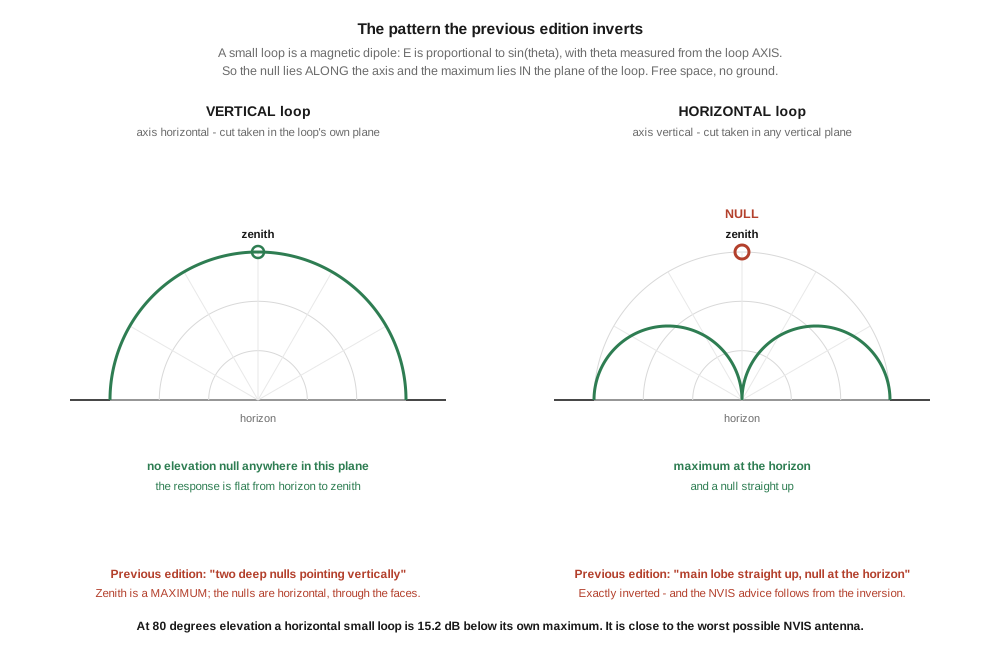
The pattern is printed upside down. §7.1 says a horizontal loop has its main lobe at the zenith and a null at the horizon. It is exactly the reverse, §2 shows why in one line of trigonometry, and the chapter’s own ASCII diagram three lines further down is correct. The NVIS recommendation built on the inverted pattern falls with it — and §2 finds that the correct NVIS orientation is the very one the chapter recommends for DX.

The noise rejection is credited to a mechanism that cannot produce it. The chapter says the loop rejects vertically polarised noise by 6 to 10 dB, in a section three pages after it correctly states that a vertical loop is vertically polarised. §5 separates the two real mechanisms from the folklore, and finds that one of them is worth far more than 10 dB and the other worth nothing, depending on a distinction the chapter never draws.

There is no exposure calculation anywhere in the chapter, which recommends this antenna for a balcony, an attic, a windowsill and a hotel room. §6 performs one. The compliance distance for the antenna the chapter specifies, at the power it specifies, is a little over two metres for a continuous carrier — and that result is confirmed independently against a published QST figure for the same antenna.

And a measured loop turns out to say something none of the first three volumes could. §7 works from Jim Ford N6JF’s portable loop in Nuts and Volts, whose published bandwidths are the only first-hand measurements available to this dive. They are much wider than the model predicts, in a pattern that identifies which component is responsible. The answer changes the practical advice, because it is not the one Vols 1 and 2 spend their time optimising.

4.2 The pattern, and the sentence that inverts it

A small loop is a magnetic dipole. Its far field is

E ∝ sin θ

where θ is measured from the loop’s axis — the normal to the plane of the loop, the direction a drill through the middle of it would point. That single line settles every orientation question in this section, and it has two immediate consequences: the null lies along the axis, and the maximum lies everywhere in the plane of the loop.

§7.1’s opening sentence states precisely that, and is correct. What follows it is not.

Table 1 — 2. The pattern, and the sentence that inverts it

The previous edition says	What the sine law gives
vertical loop: “two deep nulls pointing vertically (up and down)”	🔴 the zenith is a maximum. A vertical loop’s axis is horizontal, so straight up lies in the loop’s plane at θ = 90°. Its nulls are horizontal, out through the two faces
horizontal loop: “Main lobe pointing straight up (zenith), null at the horizon”	🔴🔴 exactly inverted. A horizontal loop’s axis is vertical, so the zenith is at θ = 0 — a null — and the maximum is at the horizon
horizontal loop: “Useful for NVIS (near-zenith) HF receive”	🔴 follows from the inversion, and is therefore also wrong. A horizontal small loop nulls straight up, which is the one thing an NVIS antenna must not do

⭐⭐ And the previous edition’s own ASCII diagram, three lines below the first of those rows, is correct — “main lobes East and West (along the loop plane), deep nulls North and South (perpendicular to loop).” That is the sine law drawn properly, sitting immediately beneath prose that contradicts it.

🔴 This is the third dive in this program with that exact shape. The antenna tuners dive had the correct L-network rule stated in plain language between two schematics that violated it, and the random wire dive drew a 9:1 transformer beside arithmetic for a 49:1. The pattern is consistent: the drawing is right, the prose is wrong, and a reader follows the prose.

4.2.1 The NVIS recommendation is backwards twice over

The interesting part is not that the NVIS advice fails. It is which orientation actually works.

Polarisation follows the same geometry. The electric field lies along m × r̂, so for a vertical loop whose axis runs north–south:

• Toward the east, in the plane of the loop: E is vertical. This is the familiar result, and it is why a vertical loop is described as vertically polarised.
• Toward the zenith: E is horizontal, running east–west.

So a vertical loop is at full amplitude straight up — §2 established the zenith is a maximum for that orientation — and is horizontally polarised when it gets there. Strong, high-angle, horizontally polarised radiation is the definition of an NVIS antenna.

⭐⭐ The previous edition recommends the horizontal loop for NVIS and the vertical loop for DX. The vertical loop is the NVIS orientation, and the horizontal loop is the only orientation that cannot do NVIS at all. Quantified: at 80 degrees elevation a horizontal small loop is 15.2 dB below its own maximum.

⚠ Do not read that as a recommendation to use a small loop for NVIS. It is a claim about orientation only. A small loop on 80 m is a couple of per cent efficient (Vol 1 §5), and a low dipole beats it comfortably wherever one will fit. The point is narrower and more useful: if a loop is what you have, the vertical orientation is the one that puts power where NVIS needs it, and the chapter tells you to do the opposite.

4.3 The null, and how accurately it must be aimed

The nulls are the small loop’s genuinely distinctive feature, and the previous edition mentions them without ever quantifying the one property that decides whether they are usable: how wide they are.

Rejection at an angle φ off the null axis is 20 log₁₀(sin φ).

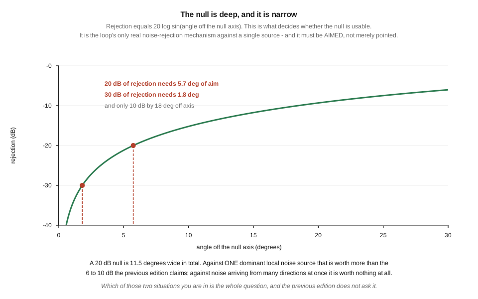
Table 2 — 3. The null, and how accurately it must be aimed

rejection	angle off the null axis	total width of the notch
10 dB	18.4°	36.9°
20 dB	5.7°	11.5°
30 dB	1.8°	3.6°
40 dB	0.6°	1.2°

⭐ A 20 dB null is 11.5 degrees wide in total. That is the number that matters, and it cuts both ways. It is deep enough to be worth having — far more than the 6 to 10 dB the previous edition claims for its noise rejection — and narrow enough that it must be genuinely aimed. Rotating a loop by hand until the noise drops finds a 20 dB null easily; holding one on a moving target, or nulling one source without swinging another into the maximum, is a different proposition.

⚠ Two practical limits keep the deep end of that table theoretical. Feedline common-mode current fills in the null — any current on the outside of the coax radiates from a different place with a different pattern, and the sum has no true zero. Ford’s article describes checking for exactly this, by running a hand along the coax near the connector and watching for SWR movement. And a null is a three-dimensional cone, not a line: ground reflections arrive from a different direction than the direct path, so an interferer that is nulled directly may still arrive by reflection.

4.4 Height, ground, and why a loop tolerates being low

A vertical loop is a horizontal magnetic dipole, and a horizontal magnetic dipole images co-directionally in a conducting ground — in phase, not reversed. The loop and its image behave as two in-phase sources separated by twice the height:

AF(ψ) = 2 cos(k h sin ψ)

At the horizon, ψ = 0, and the array factor is 2 for any height whatsoever. The horizon is reinforced no matter how low the antenna is.

That is the opposite of a horizontal dipole’s behaviour, where the image is reversed and low mounting cancels the low-angle radiation. It is the reason a magloop on a tripod a metre off the ground behaves sensibly while a dipole at the same height is a cloud-warmer.

Working the first elevation null:

Table 3 — Working the first elevation null

height on 40 m	in wavelengths	first elevation null
0.5 m	0.012 λ	none below zenith
2 m	0.048 λ	none below zenith
10 m	0.238 λ	none below zenith
10 m on 20 m	0.473 λ	31.9°

⭐ Below about a quarter wavelength there is no elevation null at all, and the pattern is a single clean low-angle lobe. Height buys a small loop far less than it buys a horizontal dipole — which is precisely why the antenna suits balconies, and why the previous edition’s stealth case is sound even where its physics is not.

🔴 One caveat, and the chapter would be wrong to omit it. That is a perfect ground. Real earth attenuates the vertically polarised reflection badly near the pseudo-Brewster angle, so the low-angle lobe is real but lossier than the array factor suggests. The loop escapes ground loss in its feedpoint budget, not in its far-field reflection, and those are different things. Vol 1 §6 makes the first point — the loop wins over a short dipole because it needs no return path — and it would be an over-reading to conclude the loop is indifferent to the ground beneath it. It is indifferent to needing a ground system. It is as subject to reflection loss as any other vertically polarised antenna.

⚠ Nearby metal is a separate matter and it does detune the loop, as Vol 1 §6 notes. The previous edition’s companion-gear advice to use a non-metallic mast is correct, and Ford’s build follows it — a PVC tripod, chosen because “the less metal in the RF field, the better.”

4.5 What the noise claim actually is

The previous edition makes the same claim twice, in §9 and again in §15:

the magnetic-field-dominant pattern of the small magloop rejects vertically-polarized noise from local sources (switching power supplies, plasma TVs) by 6–10 dB relative to a vertical antenna

🔴 This cannot be right as stated, and the chapter itself supplies the refutation. §7.1 says a vertical loop has “vertical polarization (the radiated E-field is vertical because the current is horizontal)” — which §2 confirms. An antenna cannot reject the polarisation it transmits. A vertically polarised loop is maximally sensitive to vertically polarised noise arriving in its plane. The number is attached to a mechanism that does not exist.

Two real mechanisms do exist, and separating them is more useful than the figure ever was.

The rotatable null (§3). Against a single dominant local source, the null is worth 20 dB with six degrees of aim and 30 dB with two — considerably more than the claimed 6 to 10. Against noise arriving from many directions at once, it is worth nothing at all, because a notch 11 degrees wide removes an eleven-degree slice of a full circle. Which of those two situations you are in is the entire question, and the previous edition never asks it.

Near-field wave impedance. Close to an electrically small, high-impedance noise source — a switching supply and its lead — the wave impedance is far above the 377 ohms of free space, so the electric field dominates the magnetic one. A magnetic antenna is under-coupled to that source in the same ratio:

Table 4 — Near-field wave impedance. Close to an electrically small, high-impedance noise source — a switching supply and its lead — the wave impedance is far above the 377 ohms of free space, so the electric field dominates the magnetic one. A magnetic antenna is under-coupled to that source in the same ratio

distance from the source, in kr	wave impedance	relative to free space
0.05	7525 Ω	+26.0 dB
0.10	3749 Ω	+20.0 dB
0.20	1849 Ω	+13.8 dB
0.50	695 Ω	+5.3 dB
1.00	377 Ω	0.0 dB

⭐ That is where the folklore figure comes from, and at kr around 0.1 it is worth about 20 dB. But it is a property of proximity, not polarisation — it applies only inside the reactive near field of the source, which at HF is a few metres, and it vanishes entirely for noise that has propagated any distance. A loop is quieter than a vertical against the switching supply in the next room. It is not quieter against the band.

4.6 RF safety: the calculation the previous edition never does

The chapter recommends this antenna for a balcony, an attic, a windowsill and a hotel room. It discusses capacitor arcing at length. It contains no exposure calculation of any kind.

The loop’s near field is computed here from the exact expression for a circular current loop — elliptic integrals, not the point-dipole approximation, because inside about a metre and a half the point-dipole form understates the field by up to a factor of 1.9 and would flatter the answer exactly where it matters.

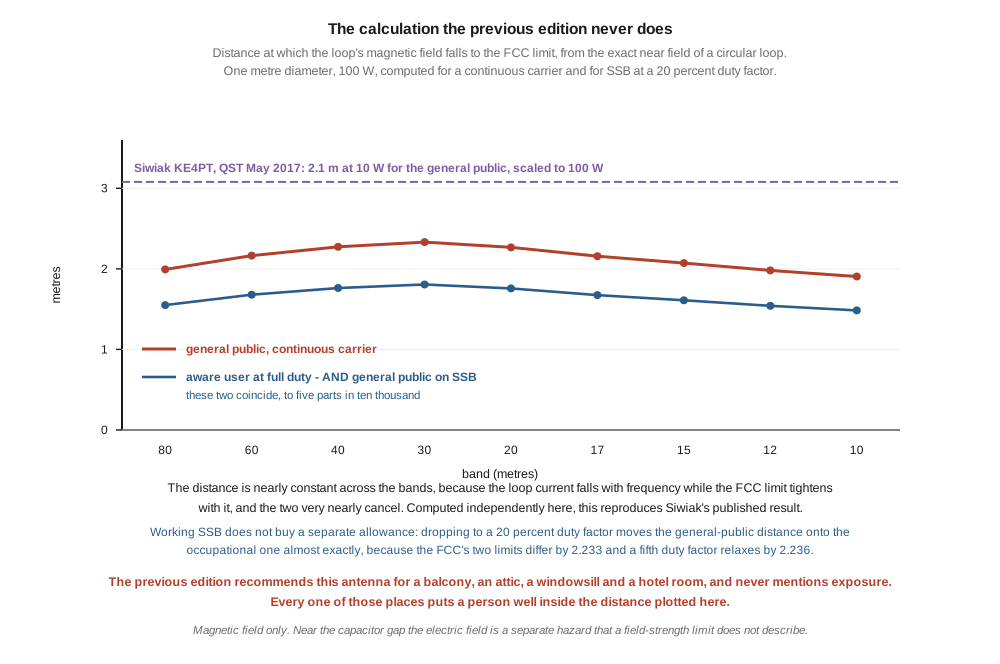
For the 1 m loop the previous edition specifies, at the 100 W it specifies, with a continuous carrier:

Table 5 — For the 1 m loop the previous edition specifies, at the 100 W it specifies, with a continuous carrier

band	H at 1 m	FCC general-population limit	times over	compliance distance
80 m	6.09 A/m	0.600 A/m	10.2×	1.99 m
40 m	4.70 A/m	0.306 A/m	15.3×	2.27 m
30 m	3.59 A/m	0.216 A/m	16.6×	2.33 m
20 m	2.35 A/m	0.154 A/m	15.2×	2.27 m
10 m	0.68 A/m	0.077 A/m	8.8×	1.90 m

⭐ The distance is nearly constant across the bands — 1.90 to 2.33 metres, a 23 per cent spread over nine bands — and the reason is worth stating because it is not obvious. Loop current falls with frequency as radiation resistance climbs, while the FCC limit tightens with frequency as 2.19/f. The two very nearly cancel.

4.6.1 An independent check, and it holds

That result can be tested against published work. Ford’s article quotes Kai Siwiak KE4PT’s QST Technical Correspondence of May 2017:

Additionally, for a one meter diameter loop operating at a continuous 10W, including ground reflection, compliance distances are nearly constant over the 40-10 meter bands at less than 1.5 meters (4.9 feet) for the aware user, and 2.1 meters (6.9 feet) for the general public.

⚠ That is Siwiak quoted by Ford; the QST original has not been read for this volume, and the volume says so rather than implying first-hand access to it. The BALUNs dive had to make the same disclosure about a Maxwell citation, and the discipline is the same one.

The same antenna, so the comparison is real. Three things to check:

1. Near-constancy over 40 to 10 metres. Computed independently here: 1.34 to 1.62 m at 10 W, a 21 per cent spread. Confirmed.
2. The distances. His figures include a ground reflection; mine do not. A perfect ground doubles the field in the worst direction, which multiplies distance by the cube root of two. Carrying that: 2.04 m against his 2.1 m for the general public, and 1.60 m against his “less than 1.5 m” for the aware user — the second landing on the correct side of a stated upper bound.
3. Scaling to 100 W. Field goes as the square root of power and falls as the cube of distance, so distance goes as P^(1/6) — a factor of 1.47 for ten times the power. His 2.1 m at 10 W becomes 3.08 m at 100 W. Ford draws the same conclusion in his own words: “Others have suggested even more distance … certainly with 100W.”

⭐⭐ An independent calculation reproducing a published figure to within a few per cent is the strongest form of confirmation this program gets, and it is the third time in this hub — after G3TXQ’s doublet in the antenna tuners dive and W9CF’s table in Vol 3 of the same — that a result has been arrived at twice by different routes.

4.6.2 The duty-factor coincidence

Dropping from a continuous carrier to SSB at a 20 per cent duty factor relaxes the limit by the square root of five, because exposure averages on the square of the field.

⭐ The general-public distance on SSB then lands on the occupational continuous-carrier distance almost exactly — to five parts in ten thousand. It is a coincidence in the FCC’s tables rather than a physical law: the occupational and general H-field limits differ by 4.89/2.19 = 2.2329, and √5 = 2.2361. But it holds across the whole 3 to 30 MHz range and makes a usable rule of thumb: working SSB rather than a carrier buys you roughly the difference between the two exposure categories, and nothing more.

4.6.3 What this means in practice

🔴 Every location the previous edition recommends puts a person well inside the computed distance. A balcony is not two metres deep. A windowsill puts the operator closer than that by definition. This is not a reason to abandon the antenna — it is a reason the chapter needed a section it does not have, and it points at the specific practices that make the antenna safe: tune at low power or on receive noise, keep people at the computed distance while transmitting, and prefer intermittent modes over carriers.

Ford independently reaches the operational half of that: “Using a low power SWR analyzer or peaking receiver noise is a safe alternative to low power SWR tuning.” Note that peaking on receive noise costs nothing here — Vol 2 §2 showed the antenna is sharp enough that receive peaking is a precise tuning method in its own right.

⚠ Magnetic field only. These are H-field compliance distances, which is the binding limit near a loop. Near the capacitor gap the electric field is a separate hazard of a different kind, and a field-strength limit is the wrong tool for it — Vol 2 §4 computed 6 246 V across that gap at 100 W. That is a contact and arc hazard, not an exposure one.

4.7 A measured loop, and what its bandwidth gives away

Every number in Vols 1 through 3 comes from a model, and every one of them carries the same caveat: the model excludes capacitor ESR and joint resistance, so every efficiency is an optimistic bound. This section is the first in the dive able to say how optimistic, because it works from measurements.

Jim Ford N6JF’s “Practical Ideas for Portable Magnetic Loop Antennas” (Nuts and Volts, July/August 2018, pp. 72–76) documents a portable loop and publishes its 2:1-SWR bandwidths. His antenna is almost exactly the one the previous edition specifies: 10 feet of circumference — 0.97 m across — in 3/4 inch type M copper, joined with eight 45-degree elbows and brazed with 15 per cent silver rod specifically to keep joint resistance down, with a measured DC resistance of 1.4 milliohms. This is a carefully built loop, and that matters for what follows.

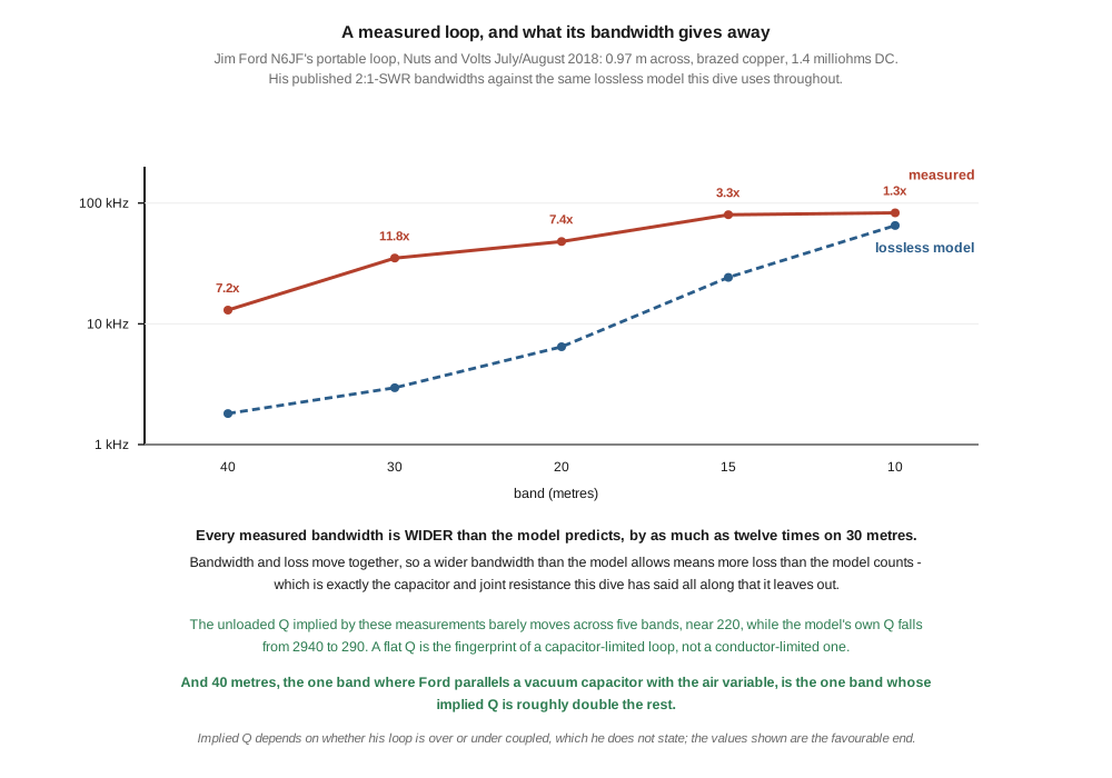
Table 6 — 7. A measured loop, and what its bandwidth gives away

band	model bandwidth	Ford’s measured	ratio	implied unloaded Q	model Q
40 m	1.81 kHz	13 kHz	7.2×	409	2940
30 m	2.96 kHz	35 kHz	11.8×	216	2563
20 m	6.45 kHz	48 kHz	7.4×	221	1641
15 m	24.2 kHz	80 kHz	3.3×	198	654
10 m	65.2 kHz	83 kHz	1.3×	228	290

Every measured bandwidth is wider than the model predicts. Since bandwidth and loss move together — Vol 1 §7’s consequence of Chu bounding Q rather than efficiency — a wider bandwidth than the model allows means more loss than the model counts. The gap is the capacitor and the joints, measured at last rather than merely acknowledged.

⚠ The implied Q depends on whether his loop is over- or under-coupled, which he does not state; the values above take the favourable branch. The unfavourable one gives Q values about 23 per cent lower still. The uncertainty runs in the direction that strengthens the conclusion, not weakens it.

4.7.1 The flat Q is a fingerprint

⭐⭐ The implied Q barely moves across five bands — 409, 216, 221, 198, 228 — while the model’s own Q falls from 2940 to 290. That flatness is the finding.

Tubing loss goes as the square root of frequency, so a conductor-limited loop’s Q rises steeply with frequency, exactly as the model column does. A capacitor with a roughly frequency-independent Q contributes a resistance X_L / Q_c at resonance, which is proportional to X_L — and that holds the loop’s Q flat. A flat Q is the signature of a capacitor-limited loop.

⭐⭐⭐ And the one band that breaks the flatness is the one band with a different capacitor. Ford runs a Johnson air variable alone on 30 through 10 metres, and parallels a 140 pF / 5 kV fixed vacuum capacitor with it for 40 metres only. Vacuum capacitors have far higher Q than air variables with wiper and frame contacts. Forty metres is the band whose implied Q is roughly double every other band’s. The one band with the better capacitor is the one band with the better Q.

⚠ That is an inference from his numbers, not a measurement he reports, and it should be read as one. But it is self-consistent, it explains both the flatness and the single outlier, and it changes the practical advice materially:

On a real portable loop the capacitor, not the tubing, is what limits efficiency. Vols 1 and 2 spend their effort on a conductor most builders have already got right.

⚠ One honest limit on the table above. Ford’s loop passes C/λ = 0.1 above 40 metres, so 20, 15 and 10 metres are outside the small-loop model’s validity (Vol 1 §2) and their implied efficiencies inherit that. Forty and thirty metres are the rows to lean on.

4.7.2 Ford’s own comparison says the same thing

At a Quartzfest demonstration he compared his loop against a commercial aluminium loop of the same size. Theirs measured 27 kHz on 40 m against his 13 kHz — and, in his words, “their extra loss could be heard by some comparing on the air signals.”

⭐⭐ Twice the bandwidth, audibly worse. That is Vol 1’s spine confirmed on the air by a third party: a loop advertising wide bandwidth for its size is advertising its losses.

⚠ And a guard against over-correcting. The implied efficiency on 40 m is around two per cent, which sounds fatal and is not. Ford reports being heard about twenty times, from Alaska to New England, on 40 m with 200 milliwatts of WSPR over about two hours. A two-per-cent antenna radiating four milliwatts still crosses a continent on a mode built for it. The finding is that the model is optimistic, not that the antenna does not work.

4.8 Operating: the signal is wider than the antenna

Vol 2 §2 established the true 2:1-SWR bandwidth. Set against the width of the signal it has to carry, one consequence stands out that neither the previous edition nor Vol 2 draws:

Table 7 — [Vol 2 §2](/transmitting-loops/vol-2/) established the true 2:1-SWR bandwidth. Set against the width of the signal it has to carry, one consequence stands out that neither the previous edition nor Vol 2 draws

band	unloaded Q	2:1-SWR bandwidth	fits an SSB channel?
80 m	2701	956 Hz	no
40 m	3147	1.61 kHz	no
30 m	2601	2.75 kHz	just
20 m	1559	6.43 kHz	yes
10 m	260	77.6 kHz	yes

🔴 On 40 and 80 metres the antenna’s 2:1 bandwidth is narrower than a single SSB channel. It is not merely a narrow antenna; it is narrower than the signal, so the edges of a transmission are presented with a worse match than its centre. Ford’s measured 13 kHz on 40 m comfortably clears an SSB channel — which is another way of seeing that his loop’s real Q is a fraction of the model’s, and a reminder that on this particular point the lossy real antenna is the more usable one.

⚠ These are model figures for the seed’s 1 m loop and are the narrowest case; a real loop with a real capacitor will be wider, for the reasons §7 gives.

Drift. The previous edition observes that a loop’s SWR drifts during operation and attributes it to “the capacitor’s plate spacing chang[ing] slightly with temperature, and the loop’s electrical length chang[ing] slightly with humidity.” Vol 2 §7 computed the mechanism that actually dominates: on 80 m the loop dissipates 98 of every 100 watts in its own tubing, heating it at 0.16 K/s and walking it half a bandwidth off frequency in about ninety seconds of continuous carrier. The drift is real; it is self-heating, not weather, and it is worst exactly where the antenna is least efficient.

⚠ The humidity effect is not zero — Ford’s capacitor arced at 100 W because a leaf had fallen on it, which is the same class of problem — but it is not the mechanism behind the drift a operator sees within a minute of keying up.

Tuning. Vol 2 §3 computed the resolution required: holding half a bandwidth on 40 m needs 47 femtofarads. That is the argument for a motor drive, and it is unanswerable — but §6 supplies a second and more urgent one. Remote tuning keeps the operator outside the compliance distance. The previous edition presents remote tuning as a convenience; it is also the safety measure.

4.9 What a small loop is actually good at

The previous edition’s best-case and worst-case lists are mostly sound, and the corrections below are narrower than the preceding sections might suggest. Where it is right, it is right.

Confirmed without qualification: the stealth and restricted-space case; field-portable operation; apartment and hotel-room work; and the observation that a horizontal dipole at 30 feet beats a vertical magloop for most HF DX, so the loop is what you reach for when the dipole is impossible.

Corrected:

🔴 The VHF dismissal is right in its conclusion and wrong in its physics. §10 says small loops at VHF are “too small (< 1 cm circumference)”. At 145 MHz a loop at the small-loop limit has a circumference of 20.7 cm — a diameter of 6.6 cm. The stated figure is off by a factor of twenty. Worse, the implied reasoning is backwards: radiation resistance climbs as the fourth power of frequency while loss resistance climbs only as its square root, so a VHF small loop is efficient — 36 per cent in 6 mm conductor, 71 per cent in 25 mm.

⭐ The real argument is simpler and survives. At 145 MHz a full-size resonant antenna is already about half a metre. There is nothing to buy with the Q. You would accept a kilohertz of bandwidth to save thirty centimetres, which is a bad trade — and that, not a fictitious size limit, is why nobody builds them.

🔴 The legal-limit voltage picks the wrong band, for the second time in the chapter. §10 says the capacitor voltage at full legal power on 80 m “can hit 15–20 kV”. For 80 m specifically that bracket is about right — the computed figure is 14 800 V. But as Vol 2 §4 established, the voltage does not peak on the lowest band. Swept across the range at 1.5 kW:

Table 8 — 🔴 The legal-limit voltage picks the wrong band, for the second time in the chapter. §10 says the capacitor voltage at full legal power on 80 m "can hit 15–20 kV". For 80 m specifically that bracket is about right — the computed figure is 14 800 V. But as [Vol 2 §4](/transmitting-loops/vol-2/) established, the voltage does not peak on the lowest band. Swept across the range at 1.5 kW

band	80 m	40 m	30 m	20 m	10 m
capacitor volts	14 800	22 362	24 192	22 157	12 826

The true worst case is 24.2 kV on 30 metres, 1.63 times the figure quoted. This is the same error as the chapter’s 100 W sizing table — it assumes the worst case lives at the lowest frequency, and it does not.

⚠ Two items are confirmed rather than corrected, since over-correction is a named failure mode in this program. The dew-and-fog warning is sound: a high-Q resonator with an exposed capacitor genuinely does degrade in damp air. And the judgement that a beverage or K9AY outperforms a transmitting loop for dedicated receive work is correct — the receive-only loops dive is the proper treatment.

⚠ One phrase to retire. §15’s myth-busting entry describes a magloop as “properly built and grounded”. Vol 1 §6 established that needing no ground system is the loop’s central virtue — the reason it beats a short dipole despite losing to it on radiation resistance by 69 times on 80 m. A loop does not want grounding; the word is a habit imported from vertical antennas.

4.10 Where this volume hands off

The small loop’s pattern is a two-line consequence of the sine law, and the previous edition prints it upside down — then builds an NVIS recommendation on the inversion, in a chapter whose own diagram three lines away has it right. The correct NVIS orientation turns out to be the one the chapter reserves for DX. Its noise-rejection figure is credited to a polarisation effect that its own polarisation statement rules out, when the real mechanisms are a null that must be aimed within six degrees and a near-field effect that dies with distance. It recommends balconies, attics and hotel rooms without ever computing an exposure distance, which is a little over two metres at the power it specifies — a figure this volume derives independently and then finds confirmed by a published QST result for the same antenna.

And a measured loop, from the one first-hand source available to this dive, says something none of the modelling could: the capacitor sets the efficiency, not the copper. A flat unloaded Q across five bands is the fingerprint, and the single band with a vacuum capacitor is the single band that breaks the pattern.

From here:

• Vol 5 — DIY build and buys builds the 1 m loop with its capacitor sized from Vol 2 §4’s voltage curve rather than from the lowest band, and now has a second reason to spend the money there: §7’s finding that the capacitor is the efficiency-limiting component. It also owes a dated, verified commercial survey — and it inherits Vol 3 §6’s warning that two of five products in the previous edition’s hex-beam list could not be found to exist.
• The receive-only loops dive is the proper home for the noise material in §5, where nulling is the design objective rather than a side effect.
• The portable and mobile monopoles dive is the comparison for the field-portable case, and shares this volume’s conclusion that a counterpoise-free antenna wins by removing a loss term rather than by radiating better.

Three things are owed. No measurement in this volume is first-hand — the bandwidths are Ford’s, the compliance figures are computed and cross-checked against Siwiak but not measured, and this dive still has no bench data of its own. The capacitor-Q inference in §7 deserves a direct test, which is a straightforward one: measure the same loop’s bandwidth with an air variable and then with a vacuum capacitor, changing nothing else. And the QST originals behind §6 should be read directly rather than through Ford’s quotation of them.

4.11 Resources

• Jim Ford, N6JF, “Practical Ideas for Portable Magnetic Loop Antennas”, Nuts and Volts, July/August 2018, pp. 72–76 — the measured loop behind §7, and the source of every bandwidth figure in it. Supplied by Jeff.
• Kai Siwiak, KE4PT, “RF Exposure Compliance Distances for Transmitting Loops, and Transmitting Loop Current”, QST Technical Correspondence, May 2017, pp. 64–65 — the published compliance distances §6 checks against. Quoted here via Ford; not read directly.
• Kai Siwiak, KE4PT, “Near Fields of an Electrically Small Loop Can Affect Direction Finding”, QST, July 2015, pp. 63–64 — cited by Ford, and directly relevant to §3’s null material.
• FCC OET Bulletin 65 and its Supplement B — the MPE limits and averaging rules used throughout §6. Ford cites Supplement B’s Table 17 for the same purpose.
• 47 CFR §1.1310 — the maximum permissible exposure limits themselves.
• ARRL Antenna Book, loop-antenna chapter — the standard treatment, and Ford’s own reference for high-voltage capacitor construction.
• Transmitting loops, Vol 1 — the fourth-power law, the validity limit marked on every figure here, and the Chu result whose consequence §7 leans on.
• Vol 2 — the bandwidth, the capacitor voltage curve, the tuning resolution and the self-heating drift referenced throughout §8.
• Vol 3 — the full-wave family, which shares a name with this antenna and nothing else.
• Antenna tuners, Vol 1 and Vol 3 — the two other places in this hub where an independent calculation reproduced a published result, and the dive whose signature defect §2 recognises here.
• Receive-only loops — nulling as a design goal.
• Portable and mobile monopoles — the field-portable comparison.