DIY Build, Measurement and Buys

---

5.1 About this volume

Four volumes of theory arrive here. Vol 1 established what a small loop costs and why it wins anyway. Vol 2 took the consequences of its very high Q — the bandwidth, the tuning resolution, the capacitor voltage and the self-heating. Vol 3 dealt with the unrelated full-wave family. Vol 4 covered pattern, siting, safety and operating, and found in Jim Ford N6JF’s measured loop the only first-hand data this dive has.

This volume builds one, and buys one.

The previous edition’s build section is the most detailed part of the chapter and the most checkable, because every number in it follows from a geometry it states. Checking them turns up four things worth the reader’s time.

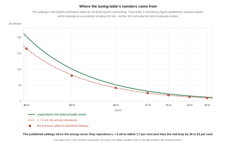
The tuning table does not describe the loop the bill of materials orders. §12.4 lists a capacitor setting for each band. Those settings reproduce an inductance of 3 microhenries to within 1.7 per cent — the figure quoted back in §3.2, which Vol 1 established belongs to a conductor of about 10 mm. Against the 3/4 inch tube this section actually orders they are 16 to 22 per cent low. One input error, four sections upstream, arriving in the table a builder uses to decide whether his antenna works.

The capacitor has a current rating, and nothing in the chapter mentions it. §3 through §11 discuss capacitor voltage at length, correctly identify it as the component that fails, and size the part from it. But a magnetic loop at 100 watts runs tens of amperes through that capacitor, and the surplus vacuum variables the chapter recommends are rated in the 40 amp region. §3 works out what the loop actually demands, and finds that the current limit and the voltage limit bind on different bands.

The commercial survey has the same trouble every survey in this hub has had. Of thirteen magnetic-loop rows, several name products that could not be found to exist, one states a band coverage its manufacturer’s own page contradicts, and the market’s most obviously current remote-tuned loop is missing entirely.

And §12.4 contains a measurement this dive has needed for five volumes without noticing. The chapter tells you to sweep the loop with a NanoVNA and check the bandwidth against a table. That sweep is not a smoke test. It is a direct measurement of the loop’s total loss resistance, and with the radiation resistance computed from the geometry it gives the efficiency — the one quantity this entire dive has been modelling and never measuring. §7 works it through, and applies it to Ford’s published numbers.

⚠ The model carried here is the same one, with the same limits. Radiation resistance is valid only for C/λ ≲ 0.1, capacitor ESR and joint resistance are excluded, and every efficiency is therefore an optimistic bound. That last exclusion stops being a caveat in this volume and becomes the subject: Vol 4 showed the excluded term is the dominant one.

5.2 Which loop is this, exactly?

Before anything can be computed, the antenna has to be pinned down, and the previous edition makes that harder than it should be. Three different conductors appear in one chapter:

Table 1 — Before anything can be computed, the antenna has to be pinned down, and the previous edition makes that harder than it should be. Three different conductors appear in one chapter

where	conductor	inductance of a 1 m loop
§3.1, the worked geometry	1 inch copper	2.358 µH
§3.2, implied by its stated L = 3 µH	about 10 mm	2.943 µH
§12.1, the build	3/4 inch (19 mm) copper tube	2.540 µH

None of these is a large error on its own — the inductances span only eight per cent either side of the middle — and it would be easy to wave the whole thing away. It matters because §12.4’s capacitor settings are computed from one of them and the builder buys another, and because the differences compound into the bandwidth and efficiency figures the same section uses as pass criteria.

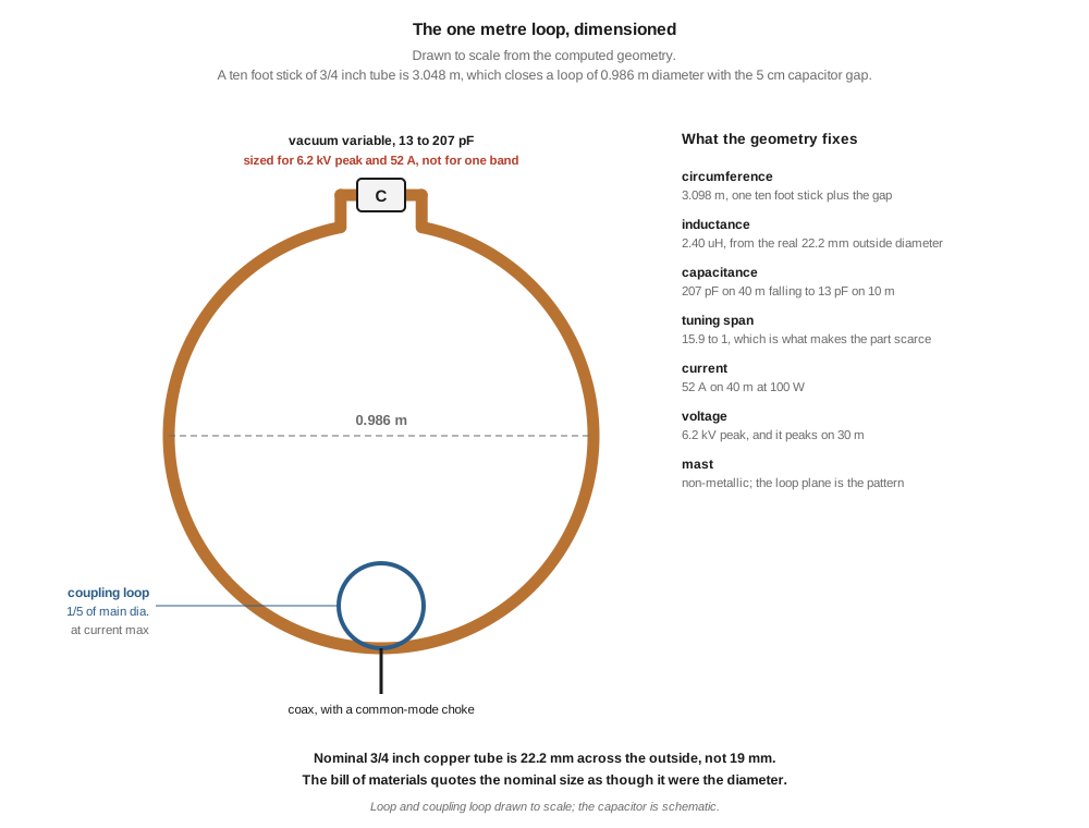
⭐ There is also a units problem in the build’s own line. North American copper tube is sized by nominal bore, and the outside diameter is one eighth of an inch larger. Nominal 3/4 inch type L or type M tube measures 22.2 mm across the outside, not the 19 mm the bill of materials puts in brackets. The parenthetical converts the nominal size as though it were the diameter. Using the real figure:

L = µ₀r[ln(8r/a) − 2] = 2.442 µH for a one metre loop of real 3/4 inch tube.

That is the number every table in this volume uses.

5.2.1 The stick will not reach

A one metre diameter loop has a circumference of 3.142 m. With the 5 cm capacitor gap §12.3 specifies, the tube itself must be 3.092 m long.

The bill of materials orders “3.5 m (1 standard length)”. There is no 3.5 m standard length. Copper tube is sold in 10 ft (3.048 m) and 12 ft (3.658 m) sticks, and the 10 ft stick — the one a builder will reach for, and the one that fits in a car — is 44 mm short of the specified loop.

⭐ The fix is to let the stick set the diameter rather than the other way round. A 10 ft length closes a loop of 0.986 m with the specified gap, which changes nothing that matters: radiation resistance falls by 5.5 per cent, efficiency by about half a percentage point on 40 m, and no other conclusion in this dive moves. Ford did exactly this, and his loop came out at 0.970 m because he used the full 10 ft as circumference.

⚠ Do not order a 12 ft stick to hit 1.000 m exactly. You will pay for and discard 566 mm of copper to buy a difference you cannot measure on the air.

5.3 The capacitor is the antenna

Vol 4 §7 established the finding this section builds on: on a real magnetic loop the capacitor, not the copper, sets the efficiency. Ford’s five measured bandwidths imply an unloaded Q that is flat across five bands where a conductor-limited loop’s Q would rise — the fingerprint of a component with roughly constant Q in series with the tubing. So the capacitor is where the money goes, and it is worth knowing precisely what it has to survive.

It has to satisfy three requirements at once, and they do not peak together.

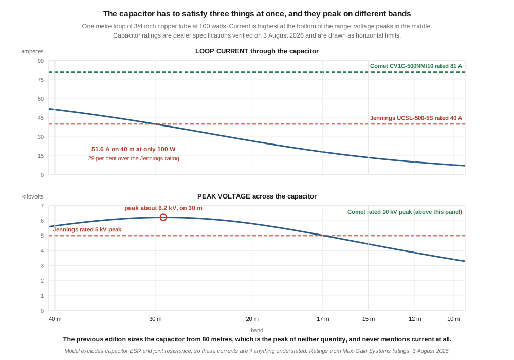
Capacitance range. From C = 1/(ω²L) with L = 2.442 µH, covering 40 m through 10 m needs 12.8 pF to 203 pF — a span of 15.9:1. This is the requirement that turns out to be hardest to buy.

Voltage. Vol 2 §4 swept this and found the peak is about 6.2 kV, on 30 metres, not on the lowest band where the previous edition sizes the part. Sizing from 80 m under-sizes by 68 per cent for this loop.

Current. I = √(P/R_total), and because R_total climbs steeply with frequency the current is highest at the bottom of the range: 51.6 A on 40 m at 100 watts, against 7.8 A on 10 m.

⭐⭐ So the capacitor meets its current limit on the lowest band and its voltage limit in the middle of the range — two different failure modes on two different bands, and the previous edition sizes for neither. It sizes voltage from 80 m, which is the peak of nothing, and it never mentions current at all.

5.3.1 What you can actually buy

The previous edition names two parts. Both need correcting, and the correction is instructive rather than fatal.

🔴 “Jennings UCSL-500-7.5” sits in a bill-of-materials row labelled “10–500 pF, 10 kV”. In Jennings’ naming the trailing number is the kilovolt rating, so the part number and the row it sits in disagree with each other by 2.5 kV before any checking. The member of that family available today is the UCSL-500-5S: 5–500 pF, 5 kV peak, 40 A RMS, $449, nine in stock at Max-Gain Systems as of 3 August 2026.

🔴 “Comet EBHC-500-10” could not be found. Comet’s variable vacuum capacitors use designations of the form CV1C, CVMN and CV05C, and a part matching the intended specification does exist — the CV1C-500NM/10, 80–500 pF, 10 kV peak, 81 A RMS, $449, out of stock at the same dealer. ⚠ Do not read this as “the part does not exist.” The class is right and the specification is right; the part number is not.

Against the loop’s three demands:

Table 2 — Against the loop's three demands

	needs	Jennings UCSL-500-5S	Comet CV1C-500NM/10
capacitance range	12.8–203 pF	5–500 pF ✅	80–500 pF 🔴 floor stops the loop at 11.4 MHz
peak voltage	6.2 kV	5 kV 🔴 short by 24 %	10 kV ✅
RMS current	51.6 A	40 A 🔴 short by 29 %	81 A ✅

⭐⭐ Neither part meets all three. Each meets two, and they fail in opposite directions. The Jennings has the tuning range and cannot take the stress; the Comet takes the stress and cannot reach past 30 metres, because an 80 pF floor on a 2.44 µH loop resonates at 11.4 MHz and no higher.

⭐⭐⭐ The way out is Ford’s, and this is the volume’s most useful practical result. He parallels a fixed vacuum capacitor with a small air variable. The fixed part carries the bulk of the capacitance — and therefore the bulk of the current — on the low bands, while the variable provides the tuning; on the high bands the fixed part is switched out and the small variable works alone, where the current is a seventh of what it was and an air variable is comfortable.

What makes this more than a plausible arrangement is that it was tested without anyone intending to test it. Vol 4 §7 found that 40 metres — the one band on which Ford parallels the vacuum capacitor — is the one band whose implied Q is roughly double the rest. The component arithmetic here and the bandwidth measurement there arrive at the same recommendation from opposite directions. ⚠ That remains an inference drawn from his bandwidth figures rather than a measurement he reports, and it is worth a direct test: the same loop, air variable then vacuum, nothing else changed.

⚠ A note on the ratings themselves. Both are steady-state RMS figures at the manufacturer’s reference conditions, and the currents above exclude capacitor ESR and joint resistance — which, as Vol 4 showed, are the dominant loss. The real current is if anything slightly lower than tabulated, because the real R_total is higher. The voltage figures move the same way. Treat the table as the right order of magnitude and the right shape, not as a specification.

5.4 The bill of materials, priced and dated

Prices verified 3 August 2026. Anything that could not be verified is marked unverified rather than filled in.

Table 3 — 4. The bill of materials, priced and dated

Part	Specification	Source	Price
Copper tubing	3/4 in type M copper, one 10 ft stick	home centre	~$35
Tuning capacitor	Jennings UCSL-500-5S, 5–500 pF, 5 kV, 40 A	Max-Gain Systems	$449
— or the higher-rated part	Comet CV1C-500NM/10, 80–500 pF, 10 kV, 81 A (40/30 m only)	Max-Gain Systems	$449, out of stock
— or QRP only	butterfly air variable, 30–300 pF	surplus	unverified
Fixed vacuum capacitor	to parallel on the low bands, per §3	surplus	unverified
Silver brazing alloy	15 % silver (Ford used Silvaloy 15)	welding supply	~$20
Coupling loop	RG-8X or #14 enamel, ~650 mm	any	~$5
Stepper motor	NEMA-17	3D-printer parts	~$25
Driver + controller	microstepping driver plus a microcontroller	various	~$25
Coax pigtail and choke	RG-8X with a mix-31 or mix-43 bead string	various	~$20
Mast and mounting	PVC or fibreglass, non-metallic	hardware	~$25
Weatherproof housing	see the note below	—	~$25

🔴 The previous edition’s own totals disagree with its own table. §12’s opening paragraph promises ”~$250 (with vacuum-variable capacitor) or ~$80 (with butterfly air-variable)”. Its bill of materials, added up, comes to $322 and $162 — out by 29 per cent and 102 per cent respectively. The section head and the table beneath it were evidently written at different times.

🔴 And the chapter contradicts itself on what a vacuum variable costs, three ways. §3.3 says “$400–1500 used”, §15 says they are “available on the surplus market for $100–300”, and the bill of materials budgets $200. A verified dealer price today is $449 for either of the two parts above. ⭐ §3.3’s bracket is the correct one; the other two are low by a factor of two or more, and the $200 line is what makes the promised $250 total possible.

⚠ §15’s underlying claim is still right, and should not be over-corrected. “Vacuum-variable capacitors are unobtainium” is indeed a myth — one dealer had nine of one part in stock on the day this was written. The myth is false; the price attached to the correction is not.

🔴 The enclosure line specifies a part that cannot do the job. The Hammond 1591 family runs from 85 × 56 × 26 mm to 190 × 111 × 61 mm; the economy 1591XX family tops out at 221 × 150 × 64 mm. The Jennings capacitor is 125.5 mm long by 58.9 mm in diameter. Allowing normal ABS wall thickness, the capacitor’s diameter exceeds the internal height of every enclosure in the 1591 series and matches the largest 1591XX to within a fraction of a millimetre — before the NEMA-17 the same bill of materials puts in the same box on the same axis, which adds a 42.3 mm body and a coupler and takes the assembly to roughly 205 mm long. ⚠ This is a sizing error, not a materials error; a weatherproof housing is genuinely needed and Vol 4’s confirmation of the dew-and-fog warning is why. Size it around the parts.

5.5 Building it

The previous edition’s step-by-step is sound in outline and most of it survives unchanged. What follows is the sequence with the corrections in place.

Form the loop. Bend the 10 ft stick into a 0.986 m circle with a 5 cm gap, over a drum or with a tube bender. Type M is thinner-walled than type L and bends more easily; the wall thickness is irrelevant electrically, because at 7 MHz the skin depth in copper is 25 µm and all of the current is in the outer surface either way.

Make the joints properly, and make as few as possible. Vol 1 put the whole antenna’s loss resistance at around twenty milliohms. A joint contributing one milliohm is a five per cent efficiency loss on its own. ⭐ Ford measured 1.4 mΩ across his finished loop and used 15 per cent silver brazing alloy rather than plumbing solder, which is the right call: silver braze has a fraction of the resistivity of tin-lead and far more of it survives thermal cycling. Soft solder in a joint carrying fifty amperes is the wrong material.

Mount the capacitor across the gap. The two tube ends turn up into the capacitor’s terminals with the shortest practical leads — every millimetre of lead is inductance in series with the tuning element and resistance in series with everything. This is the highest-voltage point on the antenna and, per §3, one of the highest-current ones.

Build the coupling loop. One fifth of the main loop’s diameter, mounted at the point opposite the capacitor. Vol 2 §5 tested the previous edition’s ratio table and found the 1/5 rule of thumb sound while the rows either side of it should not be trusted to a percentage — so treat 1/5 as a starting point and expect to adjust it. The position is right for a reason worth stating: opposite the capacitor is the current maximum, and a magnetically coupled loop wants to sit where the current is.

⚠ A note on Ford’s dimension, because it reads oddly. He describes “eight inches of RG8X” for a coupling loop he also calls one fifth of the main loop’s diameter. His main loop is 0.970 m, which is 38.2 inches, and one fifth of that is 7.6 inches — so eight inches is his coupling loop’s diameter, and it agrees with the 1/5 rule almost exactly. Making a loop of that diameter takes about 25 inches of coax. ⚠ That reading is an inference; it is not what he writes, and the alternative reading — eight inches of coax, giving a 2.5 inch loop — would be a coupling ratio of 1/15 and is inconsistent with his own description.

Fit a common-mode choke at the feedpoint. The baluns and ununs dive is the reference; the requirement is that the choking impedance be high and resistive, which is a stronger condition than “high” and the reason mix 31 or mix 43 beads are specified rather than a few turns of coax.

Mount on a non-metallic mast. This is correct as written and worth keeping. Nearby metal detunes a high-Q resonator and couples loss into it, and Vol 1 noted that a loop’s near-field immunity extends to lossy dielectrics but emphatically not to conductors.

⚠ One phrase to drop. The previous edition’s myth section describes a well-performing loop as “properly built and grounded”. Vol 4 already flagged this: needing no ground system is the loop’s central virtue. There is nothing to ground.

5.6 The tuning table, and where its numbers came from

§12.4 gives the builder a per-band table of capacitor settings and bandwidths, presented as a verification that the build succeeded. Both columns need work, and they fail for different reasons.

5.6.1 The capacitor settings

Plotted against the loop the bill of materials builds, the published settings are 16 to 22 per cent low on every band. Plotted against L = 3 µH — the figure §3.2 states — they match to 1.7 per cent mean absolute error.

⭐⭐ That is a clean diagnosis rather than seven separate errors. Vol 1 established that §3.2’s 3 µH belongs to a conductor of roughly 10 mm while §3.1 specifies 1 inch and §12.1 orders 3/4 inch. This table is the far end of that single mistake: one wrong inductance, quoted once, propagating through the capacitance formula into the numbers a builder compares his antenna against.

Corrected, for the as-built 0.986 m loop of real 3/4 inch tube (L = 2.399 µH):

Table 4 — Corrected, for the as-built 0.986 m loop of real 3/4 inch tube (L = 2.399 µH)

band	capacitor setting
40 m	207 pF
30 m	103 pF
20 m	53 pF
17 m	32 pF
15 m	23 pF
12 m	17 pF
10 m	13 pF

⚠ §3’s constraint figures are quoted for a round 1.000 m loop, to stay comparable with Vols 1 to 4. The difference between the two is under two per cent in capacitance and current and half a percentage point in efficiency — smaller than the tolerance of a hand-bent loop, and not worth carrying two sets of numbers for.

⚠ These are the settings for a bare loop in free space. Real installations shift them — a loop against a wall or in an attic sees enough nearby dielectric to move resonance by more than the tuning resolution — so the table is a starting point for finding each band, not a calibration.

5.6.2 The bandwidth column, which is subtler

The published bandwidths are labelled 2:1-SWR figures and are 2.5 to 7.3 times wider than the true 2:1 bandwidth of the loop being built. Vol 2 §2 diagnosed the general form of this — the previous edition’s §8 gives −3 dB bandwidths under a 2:1 label, a conflation this hub has now seen in a second independent seed — and the acceptance table inherits it.

⭐⭐ But here the correction needs a guard, and this is the interesting part. The lossless model says a correctly built 1 m loop shows 1.7 kHz of 2:1 bandwidth on 40 metres. Ford’s real, working, carefully built loop measured 13 kHz. The previous edition’s table says 9 kHz.

The previous edition’s number is closer to what a builder will actually measure than the corrected one is. Not because it was derived correctly — it was not — but because the loss it accidentally embodies is roughly the loss a real capacitor contributes. Publishing 1.7 kHz as the target would send a builder who measures 13 kHz looking for a fault that is not there.

🔴 The deeper problem is that the table’s direction is backwards as a quality test. Bandwidth is inversely proportional to Q, and efficiency rides on Q. A narrower measured bandwidth means a better loop. Presented as “you should see about 9 kHz”, the table tells a builder who achieves 4 kHz — a genuinely superior antenna — that he has missed the target, and reassures one who measures 20 kHz that he has hit it.

⭐ The table should give two numbers, not one: the lossless bound, which nothing can beat, and a realistic expectation for a capacitor-limited loop. For the build in this volume:

Table 5 — ⭐ The table should give two numbers, not one: the lossless bound, which nothing can beat, and a realistic expectation for a capacitor-limited loop. For the build in this volume

band	bound (best possible)	expect, at Ford’s measured Q
40 m	1.7 kHz	~20 kHz
30 m	2.8 kHz	~29 kHz
20 m	6.3 kHz	~40 kHz
15 m	24 kHz	~60 kHz
10 m	73 kHz	~81 kHz

⚠ Rows above 30 m are past the model’s validity limit and are indicative only. Note the two columns converging at the top of the range: on 10 metres the copper’s own loss has grown enough to dominate the capacitor’s, and the distinction stops mattering.

5.7 The measurement that tells you what you built

Everything above is still modelling. This section is the one that is not, and it closes a gap this dive has carried since Vol 1.

The previous edition ends its build with “test with NanoVNA — sweep 7–30 MHz, look for narrow SWR minima.” That is correct and it is a smoke test. It is also, without any additional equipment, a direct measurement of the loop’s total loss resistance — which is to say, of its efficiency.

The chain is three steps and no approximations beyond the ones already in play:

Q_u  = 0.7071 · f / BW(2:1)        measured, from the sweep
R_t  = X_L / Q_u                   X_L from the loop's geometry
eff  = R_rad / R_t                 R_rad from the geometry too

The first line is Vol 2’s bandwidth relation run backwards. The second and third need only the loop’s dimensions, which you have because you built it.

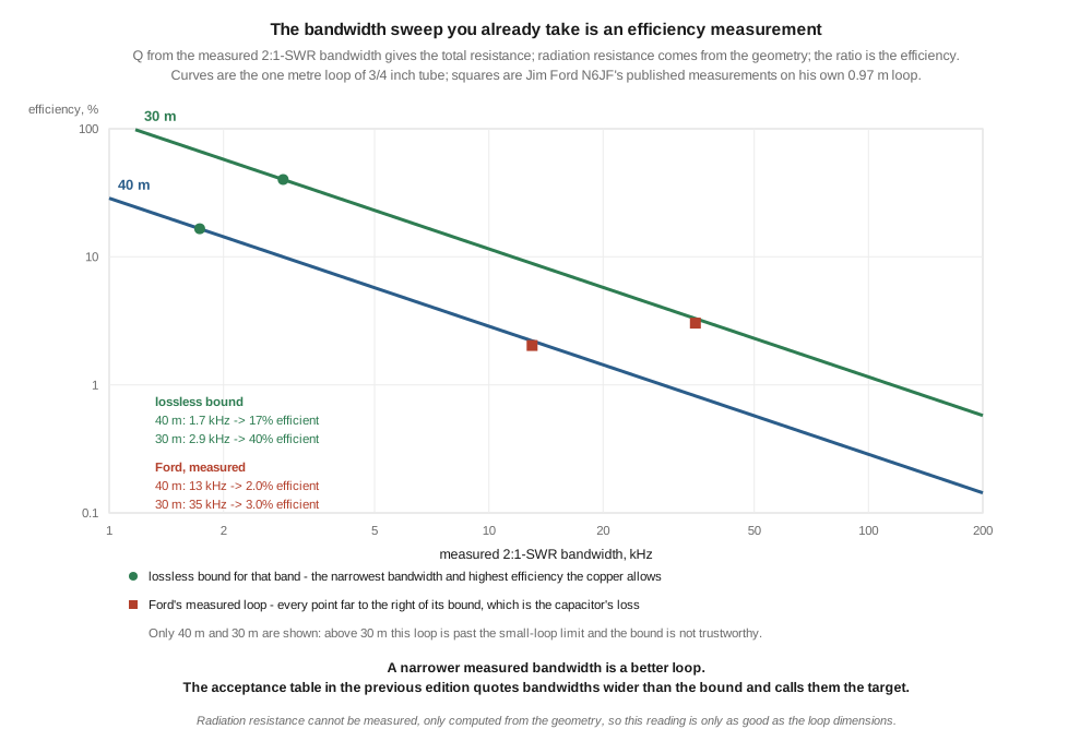
Applied to Ford’s published bandwidths on the two bands where the model is valid:

Table 6 — Applied to Ford's published bandwidths on the two bands where the model is valid

band	he measured	implied Q	implied R_total	implied efficiency	lossless bound
40 m	13 kHz	389	272 mΩ	2.0 %	15.3 %
30 m	35 kHz	205	731 mΩ	3.0 %	38.0 %

⭐⭐ This is the first efficiency figure in the dive that rests on a measurement rather than a model. It is far below the bound — by a factor of seven on 40 m — and the gap is the capacitor ESR and joint resistance the model excludes, exactly as Vol 4 inferred from the flatness of his Q.

⚠⚠ And it must not be over-corrected into a verdict on the antenna. Two per cent efficiency is −17 dB, which sounds fatal and is not: on 200 milliwatts of WSPR, that loop was heard twenty times, from Alaska to New England. Vol 1 §6 explains why an antenna this lossy is still the right choice in the space it occupies — the alternatives in the same space lose more, in a ground system instead of a capacitor.

⚠ What the measurement can and cannot tell you. Radiation resistance cannot be measured; it is computed from the loop’s dimensions. So this reading is only as good as your tape measure, and it inherits the C/λ ≲ 0.1 limit — above 30 metres on a one metre loop, R_rad itself is unreliable and the efficiency figure goes with it. Within those limits it is the most useful number a builder can extract from equipment he already owns.

⭐ Two practical uses follow immediately. Sweep the loop, change one thing, sweep again: a narrower bandwidth is a lower R_total and therefore a better antenna, with no on-air comparison needed and no reliance on propagation. And the same reading turns the capacitor question from an argument into an experiment — the direct test Vol 4 asked for is now specified: measure the bandwidth with an air variable, swap in a vacuum capacitor, measure again, change nothing else.

5.8 Driving the capacitor

Vol 2 §3 established the number that makes remote tuning necessary rather than convenient: on 40 metres, one picofarad moves the loop by about ten bandwidths. Walking to the antenna is not the problem. Resolution is.

The previous edition specifies a NEMA-17 stepper and an Arduino. ⚠ That architecture is right and should be kept. What is missing is the one number that decides whether it works.

A full step must move the capacitor by less than half a bandwidth. The Jennings UCSL-500-5S takes 21 turns for full travel over its 495 pF span, so a 200-step-per-revolution motor gives:

495 pF / (21 × 200) = 118 fF per full step

Against what the loop demands:

Table 7 — Against what the loop demands

band	half a bandwidth is	at the lossless bound	at Ford’s measured Q
40 m		49 fF	574 fF
30 m		29 fF	286 fF
20 m		24 fF	146 fF
10 m		34 fF	36 fF

🔴 Against the lossless bound a plain full-step drive is too coarse on every band — one step jumps between two and four half-bandwidths. ⭐ Against a real capacitor-limited loop it is adequate on the low bands and marginal at the top, which is the same convergence §6’s table showed and for the same reason.

⭐ One eighth microstepping gives 14.7 fF per step and clears both cases everywhere on the dial. That is a jumper on a common driver board, so the correction here costs nothing: specify the microstep setting, and the previous edition’s parts list is fine as it stands.

⚠ Two caveats. The 21-turn figure is specific to that Jennings part; other vacuum variables differ, and a butterfly air variable covers its whole range in a fraction of a turn, which makes direct drive hopeless and a reduction gearbox mandatory. And microstep positioning is not microstep accuracy — detent torque and backlash mean the achievable repeatability is coarser than the step size, which is an argument for closing the loop around an SWR reading rather than counting steps open-loop.

5.9 Buying instead: a dated survey

Every row below was checked against a manufacturer’s or dealer’s live page on 3 August 2026. Products that could not be found are listed as such rather than dropped silently, because their appearance in the previous edition is itself the finding. Prices that could not be verified are marked unverified.

🔴 The market context first: MFJ ceased manufacturing on 17 May 2024, a fact established in the antenna tuners dive and unchanged since. MFJ product pages are still live and still quote prices, and dealers still list the parts as custom-order items, but what is being sold is residual stock. The previous edition lists three MFJ loops as current.

Table 8 — 9. Buying instead: a dated survey

Model	Coverage	Power	Price	Status, 3 Aug 2026
MFJ-1786	10–30 MHz	150 W	$659.95	Live on MFJ’s store. 36 in loop. Previous edition’s $650 is close
MFJ-1788	15–40 m (7–21 MHz)	150 W	$719.95	Live. 🔴 Previous edition claims 3.5–30 MHz and 80 m capability and prices it at $1200
MFJ-1787	—	—	—	🔴 Could not be found. 404 on MFJ’s own store; absent from the product line
Chameleon CHA F-LOOP 3.0	3.5–29.7 MHz	25 W SSB / 10 W CW	from $500	Sold out on the maker’s own store
Chameleon CHA LRT (loop remote tuner)	—	—	$350	In stock. See §10
AlexLoop Walkham / Premier	7–30 MHz	20 W SSB / 10 W CW	unverified	Out of stock at GigaParts; DX Engineering’s AlexLoop brand page returns no products
Ciro Mazzoni BABY-A	40–10 m	450 W to 22 MHz, 1 kW above	unverified	Live, custom order
Ciro Mazzoni MIDI / MIDI-A	80–20 m	300 W to 8 MHz, 800 W above	unverified	Live, custom order
Ciro Mazzoni STEALTH-A	40–10 m	125 W	unverified	Live, custom order
Alpha Antenna Base MagLoop	10–40 m	100 W SSB / 50 CW / 25 digital	unverified	Live, remote-tuned. 🔴 Absent from the previous edition entirely
”CHA TIA-Mini Loop”				🔴 Could not be found
”Chameleon LOOP-30”				🔴 Could not be found
”AlexLoop ANTAL”				🔴 Could not be found
”Ciro Mazzoni Stealth Junior”				🔴 Could not be found. The real model is STEALTH-A
”NavyDavy Loop”				🔴 Could not be found
”Comrod CTL series”				🔴 Could not be found
”Magnum / Vector remote-tuning kits”				🔴 Could not be found

🔴 The MFJ-1788 error is the one that would cost a buyer money. The previous edition sells it as the 80 metre option — “3.5–30 MHz, lowest-band capable (80 m)” — and it is a 15 through 40 metre antenna on its manufacturer’s own page. Someone buying it to work 80 metres from an apartment gets an antenna that does not reach the band he bought it for. ⚠ The price error runs the other way and is the harmless direction: the quoted $1200 is 67 per cent above the manufacturer’s own $719.95.

🔴 Ciro Mazzoni’s two main models have had their coverage swapped. The previous edition gives “Baby Loop, 3.5–14 MHz”. The BABY-A is a 40 through 10 metre antenna; 80 through 20 metres is the MIDI. The bands quoted are real, and attached to the wrong product.

⭐ The omission is as informative as the errors. The Alpha Antenna base loop is a current, remote-tuned, 100 watt HF magnetic loop from a US manufacturer, and it is absent from a survey that finds room for four products that could not be found to exist. ⭐ Its power rating is also worth noting for a reason beyond the survey: 100 W SSB, 50 W CW, 25 W digital — a four-to-one spread on one antenna, rated by duty cycle in exactly the way the random wire and end-fed dive found the transformer trade does it. On a magnetic loop that spread is not only about heat in a ferrite; it is Vol 2 §7’s self-heating drift, which walks a loop off frequency in about ninety seconds of continuous carrier.

⚠ Three honest limits on this survey. Several manufacturers publish no price and route buyers through custom-order dealer pages, so the unverified rows are genuinely unverified rather than lazily so. “Could not be found” is not the same as “does not exist” — a discontinued product can vanish from search and from a manufacturer’s own store — but for a current buying guide the distinction makes no practical difference. And the whole table is dated for the reason the antenna tuners dive proved: five of five checkable prices in that chapter’s survey were wrong, and this market moves.

For the full-wave and hex-beam market, see Vol 3 §6, which surveys it and found two of five products in the previous edition’s hex-beam list that could not be found to exist.

5.10 What to avoid, and the controller that is not one

The previous edition’s “what to avoid” list is short and mostly correct. ⚠ Its three warnings are confirmed rather than corrected: cheap extruded-aluminium loops with undersized air variables do fail at the capacitor, and §3’s voltage figures say why — 3.4 to 6.2 kV at 100 watts on a part rated for a fraction of that. The scepticism about “all-band 1.5–30 MHz” claims is sound, and the reasoning given — that the loop must be physically large to reach the bottom of that range, contradicting the compactness being sold — is exactly right.

🔴 §14’s companion-gear list, though, recommends a product that cannot do the job described. It names the CG Antenna CG-3000 as “the canonical reference unit” for SWR-monitoring auto-tune of a magnetic loop, at about $300.

The CG-3000 is a remote automatic antenna tuner: 1.6–30 MHz, 200 W, a pi network with a matching range of 12 to 1000 Ω, and a stated requirement for a wire of at least 2.4 m. It is a fine unit for a random wire, an end-fed or a vertical. It cannot tune a magnetic loop, and the reason is structural rather than a matter of specification.

⭐ A magnetic loop is a resonator, not a load. You tune it by physically changing the capacitance that sets its resonance; there is nothing an external matching network can do about a loop that is off resonance except transform a very lossy impedance into 50 ohms and let the loss stand. Vol 1 put the loop’s total resistance at around twenty milliohms — a match the CG-3000’s 12 Ω floor does not reach by nearly three orders of magnitude — and in any case the coupling loop already presents roughly 50 Ω when the loop is resonant. The tuner would be solving a problem the antenna does not have, while leaving the one it does have untouched.

⭐ The product that belongs in that slot is real and is made by a manufacturer already in the survey: Chameleon’s CHA LRT, the Loop Remote Tuner, $350 and in stock. That is a device that drives the loop’s own tuning element, which is what the job requires.

⚠ One further item to treat carefully. The previous edition’s myth list says a magnetic loop “works better than dipoles in the noise — true only on receive,” attributing it to rejection of vertically polarised noise. Vol 4 §5 dismantled that mechanism — an antenna cannot reject the polarisation it transmits — while confirming that the underlying observation is real and has two other causes. Do not buy a loop for its noise rejection without reading that section; what it rejects, and what it does not, is more specific than the folklore.

5.11 Where this volume hands off

The build in the previous edition is better than its numbers. Its geometry is sound, its construction sequence is right, its choice of a stepper and a microcontroller is right, and its instinct that the capacitor is the part to worry about is right. What it gets wrong is arithmetic, and the arithmetic all runs one way: a tuning table computed from an inductance belonging to a different conductor, a capacitor sized for the wrong band and never checked for current at all, a bill of materials whose own total contradicts its own rows, a housing that will not close around the part it names, and a survey that lists four products that could not be found while omitting a current one.

⭐⭐ And underneath the corrections there is a result this dive needed. The bandwidth sweep the chapter treats as a smoke test is the efficiency measurement all five volumes have been working without. Applied to the only measured loop available, it puts a real antenna at two per cent on 40 metres against a fifteen per cent bound — and that antenna was heard from Alaska to New England on 200 milliwatts. Both halves of that sentence are the dive’s argument in miniature: the loop is far worse than its advocates claim, and it works anyway, and the honest way to talk about it is to measure it.

The dive is complete at five volumes. From here:

• Vol 1 for the fourth-power law and the reason a loop beats a short dipole while losing to it on radiation resistance.
• Vol 2 for the bandwidth, the tuning resolution and the voltage curve this volume sizes hardware from.
• Vol 3 for the full-wave family, and for the hex-beam and quad market this volume deliberately does not repeat.
• Vol 4 for pattern, siting, RF exposure and Ford’s measurements.
• The receive-only loops dive where nulling is a design objective rather than a side effect.
• The antenna tuners dive for the matching-network treatment, and for the survey whose five-of-five wrong prices set the standard this section tried to meet.
• The baluns and ununs dive for the common-mode choke, and for why “high impedance” is not a sufficient specification.

Four things are owed, and they are the same four the dive has been accumulating.

No measurement in this dive is first-hand. Ford’s numbers are the only measured data in five volumes, and they arrive via a magazine article. The loop in §5 has not been built here.

The capacitor inference deserves its direct test, and §7 now specifies it precisely enough to run in an afternoon: sweep, swap the capacitor, sweep again.

No volume in this dive has had an independent accuracy review. Author and checker have been the same throughout, which every earlier dive in this program has found to be the weaker arrangement — a fresh reviewer has found real defects in every volume of every previous dive.

And the unverified prices in §9 should be closed when the manufacturers who route through custom-order pages can be reached directly.

5.12 Resources

• Jim Ford, N6JF, “Practical Ideas for Portable Magnetic Loop Antennas”, Nuts and Volts, July/August 2018, pp. 72–76 — the measured loop behind §3, §5 and §7, and the source of every bandwidth figure in them. Supplied by Jeff.
• Max-Gain Systems vacuum capacitor listings — the Jennings UCSL-500-5S and Comet CV1C-500NM/10 specifications, dimensions, turn count, prices and stock, verified 3 August 2026.
• MFJ Enterprises product pages for the MFJ-1786 and MFJ-1788 — the coverage and prices in §9, and the absence of the MFJ-1787.
• Chameleon Antenna loop-antenna catalogue — the CHA F-LOOP 3.0 and the CHA LRT, verified 3 August 2026.
• Ciro Mazzoni automatic magnetic loop listings via DX Engineering — the BABY-A, MIDI, MIDI-A and STEALTH-A coverage and power ratings.
• CG Antenna CG-3000 documentation — the pi-network topology, 12–1000 Ω matching range and minimum wire length behind §10.
• Hammond Manufacturing 1591 and 1591XX enclosure ranges — the dimensions in §4.
• ARRL Antenna Book, loop-antenna chapter — the standard treatment, and Ford’s own reference for high-voltage capacitor construction.
• AA5TB small-loop calculator — the community’s usual design tool, and a useful cross-check on the inductance and capacitance in §2 and §6.
• Transmitting loops, Vol 1 · Vol 2 · Vol 3 · Vol 4.
• Antenna tuners, Vol 5 — the MFJ manufacturing date, and the commercial-survey standard.
• Random wire and end-fed, Vol 5 — duty-cycle power ratings, and the DIY-section defect class this volume was checked against.
• Baluns and ununs, Vol 3 — the common-mode choke.
• Receive-only loops — nulling as a design goal.