Full-Wave Loops

---

3.1 About this volume

Vols 1 and 2 were about an antenna a metre across with a Q of three thousand, two per cent efficiency on 80 metres and a bandwidth measured in hundreds of hertz. This volume is about an antenna eighty metres of wire long, with a Q around fifty, dipole-class efficiency and a bandwidth of hundreds of kilohertz.

They share the word “loop” and a chapter heading, and that is the extent of it. Nothing computed in the first two volumes applies here — not the fourth-power law, not the capacitor, not the femtofarad tuning resolution, not the 6 kV. §2 makes the comparison explicitly, because the single most common error about loops is treating a statement about one family as a statement about the other, and the previous edition’s decision to put both under one heading is the main reason that happens.

Three things in this volume correct the previous edition.

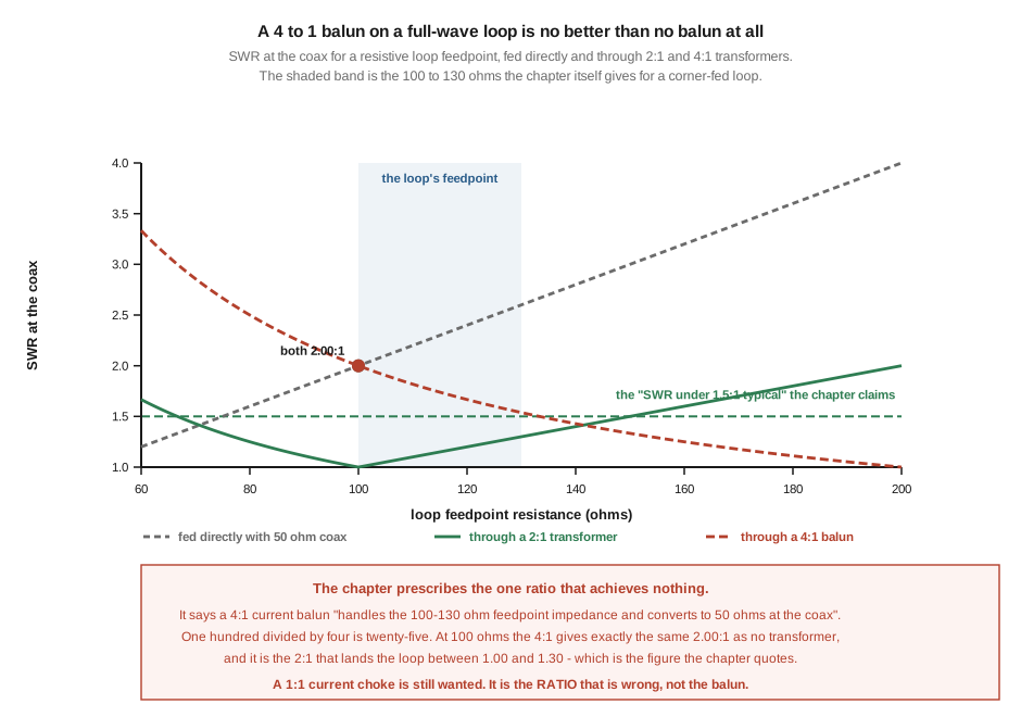
The matching prescription is wrong, and wrong in a way that is easy to check. It says a corner-fed loop’s 100–130 Ω feedpoint is handled by “a 4:1 current BALUN — the BALUN handles the 100–120 Ω feedpoint impedance and converts to 50 Ω at the coax.” One hundred divided by four is twenty-five. §4 works it through: at 100 Ω a 4:1 gives exactly the same 2.00:1 SWR as no transformer at all, and it is the 2:1 that lands the loop at 1.00–1.30:1 — which is the figure the same paragraph claims to achieve.

It never says how big the antenna is. There is no length formula anywhere in the chapter. §3 supplies it and works out the dimensions, because for this family the size is the decision.

And the hex-beam section has its inventor’s callsign wrong and a commercial survey with at least two products that do not appear to exist. §6 rebuilds it.

3.2 A different antenna with the same name

The previous edition’s own three-regime table, corrected in Vol 1 §2, already contains the distinction. Below about C/λ = 0.1 a loop carries near-uniform current and behaves as a magnetic dipole. At C/λ ≈ 1 it carries a full standing wave and behaves as a resonant current-element antenna — a folded dipole bent into a closed shape, essentially.

Everything follows from that.

Table 1 — 2. A different antenna with the same name

	small magnetic loop	full-wave loop
circumference	≈ λ/30 to λ/10	≈ λ
current	near-uniform	standing wave, maxima and nulls
feedpoint	milliohms, tuned by a capacitor	100–130 Ω, resonant
Q	250 to 3 000	tens
tuning	a capacitor, per QSY	none; cut it and leave it
efficiency	2 % to 40 % on the low bands	dipole-class
size on 40 m	1 m across	43 m of wire

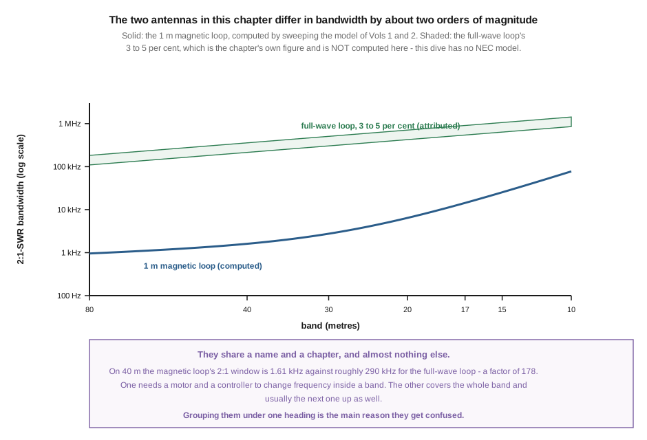
The bandwidth gulf is the sharpest single measure. On 40 metres the magnetic loop’s 2:1-SWR window is 1.6 kHz; a full-wave loop’s is a few hundred kilohertz. That is a factor of roughly 180.

⚠ An honesty note about that figure. The magnetic-loop curve is computed by sweeping the model of Vols 1 and 2. The full-wave figure of 3–5 % is the previous edition’s own number, which is consistent with the amateur literature but is not computed here — this dive has no NEC model and will not pretend to one. The two are drawn differently on the chart for that reason. The conclusion is robust to a wide margin of error in the attributed figure; the exact ratio is not.

What that means practically: one antenna needs a motor and a controller to move across a band, and the other covers the whole band and often the next one up. If you have read a claim about “loops” and cannot tell which family it refers to, the bandwidth will tell you immediately.

3.3 How big it actually is

The previous edition describes full-wave loops as “wires of total length ≈ λ shaped into a closed planar geometry” and never gives a formula. For an antenna family whose defining practical characteristic is its size, that is the omission that matters most.

The resonant length is close to, but not exactly, a free-space wavelength — the wire is thicker than nothing, near ground, and surrounded by objects, all of which slow it. The usual amateur rule is

total wire length (feet) ≈ 1005 / f(MHz)

which is 306.3 / f(MHz) metres, about 2.2 % longer than a free-space wavelength. Treat it as a starting point and trim to resonance; the environment moves it more than the formula’s precision does.

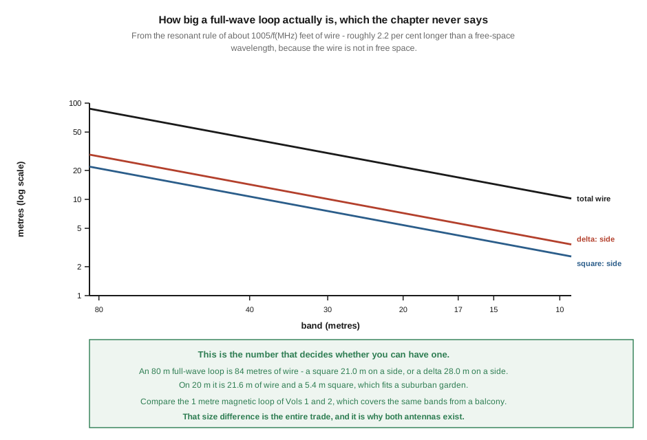
Table 2 — 3. How big it actually is

band	total wire	square, per side	delta, per side
80 m	83.9 m	21.0 m	28.0 m
40 m	42.8 m	10.7 m	14.3 m
30 m	30.3 m	7.6 m	10.1 m
20 m	21.6 m	5.4 m	7.2 m
15 m	14.4 m	3.6 m	4.8 m
10 m	10.8 m	2.7 m	3.6 m

Read the 80 m row and the trade becomes obvious. A full-wave 80 m loop is a twenty-one-metre square — four supports, each of them tall, on a plot big enough to hold it. The magnetic loop of Vol 1 covers the same band from a balcony at two per cent efficiency. That size difference is the entire reason both antennas exist, and it is a far more useful way to choose between them than any gain figure.

On 20 metres and up the calculation changes completely: a 5.4 m square is an ordinary suburban garden antenna, and there the full-wave loop stops being exotic.

3.3.1 Shape

The previous edition’s shape table is sound and worth keeping. Square, delta, diamond and rectangle all work; the choice is mechanical — how many supports you have and what fits — and it reports pattern differences under 1 dB between square and delta at the same circumference, which matches the literature.

Two additions. The delta needs the fewest supports — one apex and two corners, or a single tall support with the base guyed — which is why it dominates where trees are scarce. And the circle, which the previous edition lists as “rare — hard to construct”, is within five per cent of the delta on every dimension, so nothing is lost by ignoring it. That is why it is not on the figure.

3.4 Feeding it, and the ratio that achieves nothing

A full-wave loop’s feedpoint is resistive at resonance and, corner-fed, lands somewhere around 100–130 Ω. The previous edition’s table of feed positions is reasonable and matches the literature: corner-fed high, side-fed lower, and a mid-leg feed on a delta approaching 50 Ω directly.

Then it prescribes the transformer:

The standard configuration is corner-fed via a 4:1 current BALUN — the BALUN handles the 100–120 Ω feedpoint impedance and converts to 50 Ω at the coax. SWR < 1.5:1 is typical.

One hundred divided by four is twenty-five. A 4:1 balun steps 200 Ω down to 50 Ω; applied to 100 Ω it gives 25 Ω, and the SWR at the coax is 2.00:1.

The lead figure works all three options across the feedpoint range:

Table 3 — The lead figure works all three options across the feedpoint range

feedpoint	direct 50 Ω	2:1 transformer	4:1 balun
100 Ω	2.00:1	1.00:1	2.00:1
110 Ω	2.20:1	1.10:1	1.82:1
120 Ω	2.40:1	1.20:1	1.67:1
130 Ω	2.60:1	1.30:1	1.54:1

⭐⭐ At 100 Ω the 4:1 balun gives precisely the same SWR as feeding the loop directly with 50 Ω coax. It transforms the impedance past the target and out the other side by the same ratio it started off by. Across the whole feedpoint range it never gets below 1.54:1, and it is the 2:1 that produces the “SWR < 1.5:1 typical” the same sentence claims — comfortably, at 1.00 to 1.30:1.

3.4.1 What to actually do

Use a 2:1 transformer, which for a balanced feedpoint means a 2:1 current balun or a quarter-wave 70 Ω coaxial matching section — √(100 × 50) = 70.7 Ω, which is what 75 Ω television or CATV cable is close enough to. That matching stub is the traditional answer and it costs a few metres of cheap coax.

Or feed a delta at the middle of a bottom leg, where the previous edition’s own table puts the impedance at 50–80 Ω, and use a 1:1 choke. Simplest of all, and it is why that feed point is common on delta loops.

⚠ But do not read this as “skip the balun”. The loop is a balanced antenna and coax is unbalanced; without a choke the coax braid joins the antenna and the pattern and noise floor both suffer — which is the BALUNs and UNUNs dive’s subject and applies here in full. It is the ratio that is wrong, not the balun. A 1:1 current choke is wanted in every one of these arrangements.

⚠ And one thing the previous edition gets right that is worth keeping: it recommends a current balun rather than a voltage type, and on an antenna whose feedpoint is not perfectly symmetric — which a corner-fed loop with a real feedline never is — that is the correct choice.

3.5 Pattern, polarisation and the quiet-loop claim

A full-wave loop radiates broadside — off the two faces of the loop, like a dipole in the plane of the wire — and the previous edition’s free-space figure of about 3.0 dBi against a dipole’s 2.15 dBi is consistent with the literature. Call it a decibel. ⚠ That figure is attributed rather than computed here, for the reason §2 gives.

A decibel is not why anyone builds one. Two other properties are.

3.5.1 Polarisation is chosen by where you feed it

This is the practically useful fact, and the previous edition states it too loosely — “polarization along the feed axis” — to act on.

For a loop mounted in a vertical plane, the polarisation is set by the feedpoint’s position around the loop, because the polarisation follows the direction of the current at the point of maximum current:

• Fed at the middle of the bottom (or top) side — the current maximum is horizontal, so the loop is horizontally polarised.
• Fed at the middle of a vertical side — the current maximum is vertical, so the loop is vertically polarised.
• Fed at a corner — a diagonal current maximum, so the polarisation is diagonal and the loop has a component of both.

⭐ That means one piece of wire can be either polarisation, decided by which side you break to insert the feedline. On a delta loop it is the standard way of choosing: feed the apex or the middle of the bottom leg for horizontal, feed a third of the way up a sloping side for vertical.

And the choice matters, because a vertically-polarised loop against real ground puts more of its energy at low elevation angles, which is what long-haul HF paths want, while a horizontally-polarised one at modest height puts it high. A vertically-polarised delta loop is a classic low-band DX antenna for exactly this reason, and it gets there without the radial field a vertical monopole would need — which is the same argument Vol 1 §6 made for the small loop, appearing again in a completely different antenna.

⚠ Height still governs. No feedpoint choice rescues a horizontally-polarised loop hung at a tenth of a wavelength; it will be a cloud-warmer whatever you do. The single-band dipole dive has the height-against-take-off-angle relationship, and it applies to a horizontally-polarised loop essentially unchanged.

3.5.2 The quiet-loop claim, which does not transfer

The previous edition says of full-wave loops that “the closed loop has lower local-noise pickup than an open-wire dipole because the loop’s geometry partially cancels out near-field electric noise sources”, and in its myth list allows “partly true… ~3 dB lower local-noise pickup. The effect is real but modest.”

🔴 The mechanism it gives is the small loop’s, and a full-wave loop does not have it.

Vol 1 §6 established why a small loop is tolerant of its surroundings: its stored near-field energy is overwhelmingly magnetic, and the lossy dielectrics around an indoor antenna couple far more readily to an electric field. That argument depends entirely on the loop being electrically small, so that the current is uniform and the structure behaves as a magnetic dipole.

A full-wave loop is C/λ ≈ 1. It carries a full standing wave with current nulls and voltage maxima, and it has an electric near field like any other resonant wire antenna. It does not inherit the small loop’s near-field discrimination, and quoting the same mechanism for both is exactly the category error §2 warns about.

⚠ That said, the observation is not simply wrong, and it would be an over-correction to say so. Full-wave loops do often sound quieter than a dipole in the same place, and there are two real reasons that have nothing to do with magnetic near fields:

• It is a closed, balanced structure, so with a proper current choke it is good at rejecting common-mode pickup on the feedline — and feedline pickup is a large part of what people call “local noise”. ⭐ But a dipole with an equally good choke gets the same benefit, so this is a statement about the balun, not about the loop.
• A loop is a smaller structure than a dipole for the same band in one dimension, and it is often possible to site it further from the house wiring that generates the noise. That is a siting advantage, not an electrical one.

So the honest version is: a full-wave loop is often quieter in practice, for reasons of balance and siting rather than because it is a loop. The genuinely loop-specific noise advantage belongs to the small loop, and to the receive-only loops of the companion dive — where it is the whole point rather than a side effect.

3.6 The quad and the hex beam

Two directional antennas are built from full-wave loops, and the previous edition covers them briefly and with some errors.

3.6.1 The cubical quad

A cubical quad is a parasitic array whose elements are full-wave loops rather than dipoles. The previous edition’s account of the trade is reasonable: somewhat more gain per element than a Yagi, wider bandwidth, and more mechanical complexity, wind load and volume.

⚠ The gain claim needs one qualification it does not get. “~0.5–1 dB more gain per element” is a fair description of short arrays — a two-element quad genuinely beats a two-element Yagi by around a decibel — but the advantage shrinks as boom length grows, and for long booms quads and Yagis of the same boom length perform very similarly. Quoting a per-element figure implies it scales, and it does not. The Yagi-Uda dive has the boom-length-versus-gain relationship that governs both.

Its conclusion is sound: modern LFA and OWA Yagis deliver comparable performance with less mechanical trouble, and the quad’s surviving niche is stealth — wire elements are far less visible than aluminium.

3.6.2 The hex beam

The hex beam is a compact multi-band directional antenna: wire driven and reflector elements strung on a six-arm fibreglass spider, nesting five or six bands on one frame in a turning radius small enough for an ordinary garden.

🔴 The previous edition credits it to “Mike Traffie K1WHS, 1992”. The name is right and the callsign is wrong — the hex beam is Mike Traffie, N1HXA, who developed it in the early 1990s and trademarked the term. The 1992 date is plausible but sources vary between the early nineties and 1996, so it is safer to say early 1990s than to pick a year.

🔴 And the chapter omits the development that produced the version most people now own. In 2008 Steve Hunt, G3TXQ redesigned the element geometry — the reflector becomes half a hexagon rather than the original’s W shape — to give substantially broader bandwidth across 20 through 10 metres. K4KIO’s QST article in early 2009 popularised that topology. The “broadband hexbeam” that dominates the current market is the G3TXQ variant, not the original, and a chapter that names neither Hunt nor the redesign is describing a 1990s antenna as though it were the current one.

⭐ A pleasing footnote: G3TXQ is the same Steve Hunt whose transmission-line work underpins the antenna tuners dive. He turns up twice in this hub, in unrelated corners.

3.6.3 The market, and what could not be found

🔴 The previous edition’s five-product hex-beam list does not survive checking, and it fails in the way this program has now seen three times.

Table 4 — The market, and what could not be found

listed	what checking found
”K6XX Optibeam KU-3F, ~$1500”	Not found. OptiBeam is a German manufacturer, and K6XX is an unrelated US callsign. The two appear to have been welded together
”SteppIR DB6, ~$3500”	Not found as a hex beam. SteppIR’s DB-series are motorised Yagis
”MFJ-1840, ~$700”	The MFJ hex beam is the MFJ-1848, an 8-band model using the G3TXQ element configuration. 🔴 And MFJ ceased manufacturing on 17 May 2024
”MyAntennas H6F, ~$1100”	Not found
”K4KIO Hex Beam, ~$1200”	Real — KIO Technology, and the canonical DIY reference. Current pricing is $891 for all six bands and $561 single-band, so the figure quoted is high

And the makers actually found in the market — Traffie Technologies (the originator, still selling), SP7IDX, and DX Engineering — appear nowhere in the list.

⭐ This is the fabrication failure mode, and it is now the third dive to show it, after the Yagi dive’s non-existent “M2 7M9SSB” and the portable-monopole dive’s “Diamond NR-2000NMO”. The pattern is consistent: real manufacturers, real-looking part numbers, plausible prices, and no such product. A commercial survey is the part of a chapter least able to survive being written from memory, and Vol 5 treats every row of its own survey accordingly — verified against a live page, or explicitly marked unverified.

3.7 Where this volume hands off

The full-wave loop shares a name with the antenna of Vols 1 and 2 and nothing else: a hundred times the bandwidth, a hundredth of the Q, no tuning capacitor, dipole-class efficiency, and eighty-four metres of wire on 80 m against one metre across. Its size is the whole decision, and the previous edition never gives a length formula. Its feedpoint is 100–130 Ω, which wants a 2:1 transformer or a 70 Ω quarter-wave section — not the 4:1 the chapter prescribes, which at 100 Ω is arithmetically identical to using no transformer at all. And its two directional derivatives are covered with the inventor’s callsign wrong, the modern broadband redesign missing entirely, and a product list of which two entries could not be found to exist.

From here:

• Vol 4 — Choosing, siting and operating returns to the small loop for pattern and practice, and has an inversion to correct: a horizontal small loop nulls straight up, which is the reverse of what the previous edition says and undoes the NVIS recommendation built on it. It also covers the near-field and RF-safety question that 6 kV raises.
• Vol 5 — DIY build and buys builds the 1 m magnetic loop with its capacitor sized from Vol 2 §4’s curve, and surveys the market with every row dated and sourced.
• The Yagi-Uda dive is where the quad-versus-Yagi comparison in §6 properly belongs, since the governing relationship is boom length against gain.

Two things are owed. The full-wave loop’s bandwidth and gain figures in this volume are attributed, not computed — the small-loop model of Vols 1 and 2 does not reach this family, and a proper treatment wants NEC. That is a real limit on this volume and it is marked wherever it applies. And the hex-beam product survey should be re-checked against live pages before publication, since §6’s own point is that surveys rot.

3.8 Resources

• ARRL Antenna Book, loop-antenna chapter — full-wave loop dimensions, feedpoint impedance by feed position, and the quad.
• KIO Technology (K4KIO), History of the Hexbeam — the origin, Mike Traffie N1HXA’s original design, and the G3TXQ redesign. The clearest account of the lineage.
• Steve Hunt, G3TXQ, The Hexbeam Story — the 2008 broadband redesign in the designer’s own words.
• L. B. Cebik, W4RNL — the modelling work behind the quad-versus-Yagi comparison, and the reason §6 qualifies the per-element gain claim.
• Transmitting loops, Vol 1 and Vol 2 — the other family, and the source of every computed number in §2’s comparison.
• BALUNs and UNUNs, Vol 1 — why a balanced antenna on coax wants a current choke regardless of ratio, and Vol 4 for the ratios themselves.
• Yagi-Uda, Vol 2 — boom length against gain, which governs the quad comparison too.
• Antenna tuners, Vol 1 — G3TXQ’s other appearance in this hub.