Feedpoint Impedance and Matching

---

2.1 About this volume

Vol 1 fixed the geometry and the physics of the canonical half-wave element — the standing-wave current and voltage distributions, the accelerating-charge radiation mechanism, the end-effect rolled into the trim factor k ≈ 0.95, the 468/f length rule, and the 2.15 dBi directivity that makes the dipole the 0 dBd reference. This volume takes the feedpoint seriously. It owns one node of the antenna — the geometric center, where the coax meets the wire — and the entire problem of getting power across that junction cleanly.

That problem has two halves, and it is worth stating up front that they are different problems that the literature too often blurs together. The first half is the feedpoint impedance: the complex Z = R + jX the antenna presents looking into the feed terminals, where the 73 + j42.5 Ω of a free-space half-wave comes from, why trimming to resonance cancels the reactance, and how real ground at a finite height moves the resistance around. The second half is the balance problem: a dipole is an inherently balanced, symmetric structure, and coax is an inherently unbalanced one, so connecting them directly invites a third current onto the outside of the coax shield — the common-mode current that turns the feedline into part of the antenna. The impedance problem is, for a resonant dipole on 50 Ω coax, almost a non-event; the balance problem is the one that actually degrades real installations, and the 1:1 current balun that solves it belongs at every dipole feedpoint without exception.

Stay aware of the volume boundaries. The static impedance picture — the value of Z at and near resonance, and how it varies with height — is this volume’s. The way that impedance sweeps with frequency, the resulting SWR-versus-frequency curve, the antenna’s bandwidth and Q, and the radiation-pattern consequences of height all belong to Vol 3 and are forward-referenced rather than pre-empted here. The hands-on winding of a balun, the bench measurement of its choking impedance, and the trim-and-sweep tuning loop are Vol 5. What this volume establishes is the electrical reasoning: what the feedpoint looks like, why the 50 Ω mismatch does not matter, and why the choke is non-negotiable.

2.2 The free-space feedpoint: 73 + j42.5 Ω

A thin, lossless half-wave dipole in free space, cut to exactly a free-space half-wavelength (L = λ/2, before any end-effect trim), presents a feedpoint impedance very close to

Z_fp ≈ 73 + j42.5 Ω.

This is the canonical figure from the antenna literature — Balanis derives it from the induced-EMF method, integrating the near-field reaction of the sin(βz)/cos(βz) current distribution against itself, and it is reproduced in every edition of the ARRL Antenna Book. Both parts of that complex number have a clean physical reading, and understanding them is the whole of the impedance story.

The real part, ≈ 73 Ω, is the radiation resistance — the equivalent resistance that, carrying the feedpoint current, would dissipate the same power the antenna actually radiates into space. It is not a loss in the ohmic sense; it is the “resistance” that radiation looks like to the source, and it is what couples the transmitter’s power into the far field. Section 3 develops it properly.

The imaginary part, +j42.5 Ω, is inductive reactance, and it is present for exactly the reason Vol 1 gave when it distinguished electrical from physical length: a wire cut to a full free-space λ/2 is electrically slightly too long to be resonant. The end-effect — the shunt capacitance at the high-voltage tips — makes the element behave as though it were a little longer than it physically is, pushing it just past the resonant length, and an element just past resonance looks inductive. The +j42.5 Ω is the signature of that small excess length. This closes the loop with Vol 1’s trim factor exactly: trimming the element by the few percent that takes k from 1.0 down to ≈ 0.95 is the same act as tuning the reactance out. When you shorten a full-λ/2 element to its resonant length, the inductive +j42.5 Ω walks down toward zero, and at resonance the feedpoint is purely resistive.

There are, in principle, two ways to dispose of the +j42.5 Ω. You can trim the wire shorter to bring the resonant length down until X = 0 — the standard approach, mechanical and permanent, and the entire reason the cut-to-length apparatus of Vol 1 exists. Or you can leave the wire long and cancel the reactance electrically with a series capacitor of the right value at the feedpoint, or with a tuner. Almost nobody does the second for a single-band dipole: a capacitor at the feedpoint is one more outdoor component to weatherproof and one more thing to fail, and trimming the wire is free and stays put. So the practical sequence is the one Vol 1 described — cut, hoist, sweep, trim — and the endpoint of that sequence is a feedpoint that, in free space, sits at

Z_fp ≈ 73 + j0 Ω.

A subtlety worth stating, because it shows up on a careful sweep: shortening the element to cancel the reactance also pulls the resistance down slightly, so a resonant thin dipole is often closer to 70 Ω than to the textbook 73 Ω. The difference is within the scatter of any real installation and is swamped by the ground effect of the next section, but it is the reason measured resonant dipoles cluster a hair below 73 Ω rather than exactly on it. Vol 3 shows how this same reactance, viewed as a function of frequency rather than length, becomes the SWR curve.

2.3 Radiation resistance — what the 73 Ω actually is

The radiation resistance R_r is the bridge between the field picture and the circuit picture, and it repays a careful definition. If the antenna radiates a total power P_rad and carries a current I at the reference point, then by definition

R_r = P_rad / |I|² (using RMS current),

so that the radiated power can be written P_rad = |I|² R_r exactly as if R_r were an ordinary resistor. The crucial qualifier is the phrase at the reference point, because the current on a dipole is not uniform — it is the half-cosine of Vol 1, maximum at the center and zero at the ends. Radiation resistance therefore depends on where you reference the current, and the conventional choice for a center-fed half-wave is the current maximum, which is the feedpoint. Referenced there, a thin half-wave dipole has R_r ≈ 73 Ω. (Referenced to the current at the ends, where the current is zero, the radiation resistance would be infinite — a reminder that the number is meaningless without its reference point. The “73 Ω” you feed is specifically the current-maximum value.)

It is essential not to confuse radiation resistance with the wire’s ohmic resistance. The ohmic part is genuine I²R loss — copper heating, skin-effect resistance, connector and joint resistance — and it is what determines radiation efficiency. For a full-size copper HF dipole that ohmic resistance is a small fraction of an ohm against a 73 Ω radiation resistance, so the efficiency is essentially 100% and effectively all the power the transmitter delivers to the feedpoint is radiated. This is why Vol 1 could treat the dipole’s 2.15 dBi directivity as interchangeable with gain: there is almost no loss for the directivity to be discounted by. The distinction only bites for shortened or heavily loaded elements (loading coils, capacity hats, short mobile whips) where the radiation resistance collapses to a few ohms or less and the fixed ohmic and coil losses become a large fraction of the total — those are the antennas where efficiency is a live problem, and they live in other dives. For the full-size half-wave that is this dive’s subject, R_r ≈ 73 Ω is the feedpoint resistance to within a fraction of an ohm.

One more property of R_r matters for the volumes downstream: it is a property of the current distribution and the geometry, not of the feed. Bend the dipole into an inverted-V and the changed geometry changes R_r (it falls toward 50 Ω as the apex angle closes — a Vol 4 topic). Fold the element back on itself and the current splits between two conductors, stepping the feedpoint resistance up by 4× to ≈ 290 Ω while the radiation resistance referenced to the total current is unchanged — the folded dipole’s impedance transformation, also Vol 4. The 73 Ω is the canonical reference value for the straight, thin, center-fed half-wave, and the rest of the family is read as departures from it.

2.4 Feedpoint impedance over real ground

A dipole in free space is a textbook abstraction. Every real horizontal dipole hangs at a finite height above real, lossy ground, and the ground reflects the antenna’s field back up onto the wire. The cleanest way to think about it is the method of images: a perfect ground plane is electrically equivalent to a mirror-image dipole the same distance below the surface, carrying a current whose phase is set by the reflection. The real antenna’s feedpoint impedance is then its own free-space self-impedance plus a mutual-coupling term with that image — and because the image sits a distance 2h away (twice the height), the strength and phase of the coupling change continuously as the height h changes. The result is that the feedpoint resistance and reactance oscillate around their free-space values as a function of height in wavelengths, the swing largest when the antenna is low (image close, coupling strong) and damping out as the antenna rises and the image recedes.

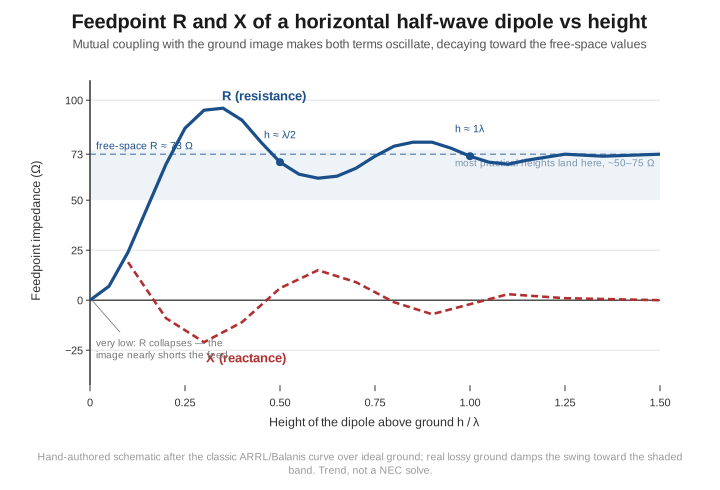
Reading the curve from the bottom up tells the practical story. At very low heights (h below roughly 0.1 λ) the image is so close and so nearly out of phase that it partially cancels the antenna’s own current; the radiation resistance collapses, heading toward zero as the antenna approaches the ground, and over real (lossy) ground that collapse is accompanied by genuine ground loss that the image model does not show. This is why a dipole strung a few feet off the ground is both low-impedance and inefficient — the close image is shorting out the feed. As the antenna rises through the region around h ≈ 0.2–0.25 λ the resistance climbs back through convenient values; this is the band where many practical HF dipoles live, and it is no accident that a dipole at a “normal” backyard height tends to present something close to 50 Ω. The resistance overshoots and peaks somewhat above the 73 Ω free-space value near h ≈ 0.35–0.4 λ, dips back through 73 Ω near h ≈ λ/2, swings again, and passes through convenient values once more near h ≈ 1 λ — the excursions getting smaller each cycle. By a height of a wavelength or two the dipole is, for impedance purposes, effectively in free space at ≈ 73 Ω.

The reactance traces a parallel oscillation. An element trimmed to be resonant in free space is not exactly resonant at every height — the same mutual coupling that moves the resistance also adds a small reactive component that swings positive and negative as the height changes, which is why a dipole re-trimmed at one height shows a small residual reactance when re-hung at another. In practice the reactive excursion at normal heights is modest and is trimmed out at the height the antenna will actually live at.

The single number to carry away is that most practical horizontal-dipole heights land the feedpoint resistance somewhere between about 50 and 75 Ω — the shaded band in the figure. A dipole low enough to misbehave (R falling well below 50 Ω, ground loss rising) is one strung below about 0.15 λ; a dipole high enough to sit near its clean free-space 73 Ω is one up around a wavelength. Between those extremes — exactly where backyard HF dipoles hang — the resistance stays in a band that a 50 Ω feed handles comfortably, which is the empirical justification for the next section. (The radiation-pattern consequences of these same heights — the elevation lobing, the NVIS-versus-DX trade, the peak-gain-versus-height table — are a different axis of the height story and are worked out in full in Vol 3. Here the height affects only the feedpoint impedance.)

2.5 The 50 Ω coax “mismatch” — and why it is harmless

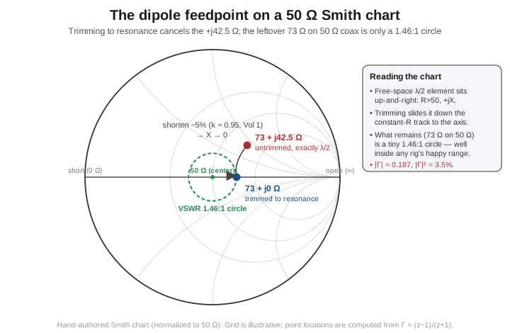
Feeding a resonant ≈ 73 Ω dipole with the 50 Ω coax that every modern station is built around is a deliberate, accepted, and almost entirely harmless mismatch. The arithmetic is worth doing explicitly because it dissolves a great deal of needless worry. The voltage reflection coefficient at the junction of a 73 Ω resistive load and a 50 Ω line is

Γ = (Z − Z₀)/(Z + Z₀) = (73 − 50)/(73 + 50) = 23/123 = 0.187,

and the standing-wave ratio is

VSWR = (1 + |Γ|)/(1 − |Γ|) = 1.187/0.813 ≈ 1.46:1.

That is the entire “mismatch” of a textbook-perfect dipole on coax: 1.46:1. The fraction of forward power reflected at the junction is |Γ|² = 0.035 — 3.5% — and the rest is accepted by the antenna on the first pass.

How much power does that cost? The pessimistic bound is the mismatch loss — the figure you get by assuming the reflected 3.5% is simply gone:

ML = −10·log₁₀(1 − |Γ|²) = −10·log₁₀(0.965) ≈ 0.155 dB.

But that bound overstates the real loss, because the reflected power is not actually thrown away. It travels back down the line to the transmitter, where a solid-state PA’s output network (and, in the conjugate-match idealization, the source impedance) re-reflects most of it back toward the antenna for another pass; on a low-loss line the energy ends up radiated after a round trip or two. The quantity that actually measures wasted heat is the additional loss under SWR — the difference between the line’s loss with the 1.46:1 standing wave present and its loss when perfectly matched — and for the very low matched-line loss of HF coax this works out to only a few hundredths of a dB (on the order of 0.05 dB for a typical HF run). Either way you count it — 0.155 dB worst-case mismatch loss, or ≈ 0.05 dB of genuine extra dissipation — the number is a small fraction of one dB, and inaudible on the air. A 0.1 dB change is about 2% in power; no operator has ever detected it in a signal report.

The instinct to chase a perfect 1:1 comes from two places, both obsolete for this case. One is the QRP and tube-transmitter era, when output stages had narrow matching ranges and a pi-network that had to be retuned for the load; a 1.46:1 load was a real nuisance to a transmitter that wanted to see exactly 50 Ω. A modern solid-state HF radio delivers full rated power into 1.5:1 without foldback — its protection circuitry does not even begin to act until something like 2:1 to 3:1 — so a 1.46:1 dipole is invisible to it. The other source is conflating SWR with antenna performance, when SWR is purely a feed-system bookkeeping number: a dipole at 1.46:1 radiates every bit as well as the same dipole would at 1.0:1. Chasing a perfect match on a single-band HF dipole is effort spent for no measurable return.

When would a 50→75 Ω transformation earn its keep? Three honest cases. First, on a long, lossy feedline — many tens of metres of small coax, or operation up where matched-line loss is no longer negligible — where the additional-loss-under-SWR term, small per unit length, accumulates enough to matter; there, presenting the line a better match at the antenna end is worthwhile. Second, in measurement and instrumentation contexts (a 75 Ω receive distribution system, precision noise-figure work) where the match is part of the specification rather than a convenience. Third, when an installation genuinely runs at a height or in a configuration that pushes the feedpoint well away from 50 Ω — a very low dipole down at 25–35 Ω, where a 1.5:1 transformer (an unun) at the feedpoint does clean up a 2:1-or-worse SWR. For the ordinary backyard dipole at ordinary height on ordinary coax, none of these applies, and the right matching network is no network at all — just the balun of the next section.

2.6 Common-mode current and feedline radiation

If the impedance mismatch is the problem that isn’t, common-mode current is the problem that is — the dominant real-world failing of a coax-fed dipole, and the reason this volume insists on a balun. The mechanism follows directly from how current lives on a coaxial line.

A coaxial cable supports three currents, not two. There is the current on the center conductor; there is the current on the inner surface of the shield, which skin effect holds equal and opposite to the center-conductor current; and there is the current on the outer surface of the shield, which skin effect isolates almost completely from the inner two. The first two are the wanted differential (transmission-line) mode — equal, opposite, fields confined between conductor and shield, no radiation. The third is the common mode, and it has nothing to do with transmission-line operation: it is free to flow on the outside of the shield as if the shield were just another wire.

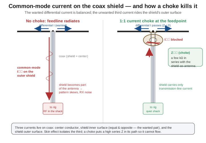
Where does the common-mode current come from at a dipole feed? From the balance mismatch. The dipole is a balanced load — two symmetric arms — and it wants to draw equal and opposite currents from its two feed terminals. Coax is an unbalanced source: one terminal is the center conductor, the other is the shield, and the shield has that extra outer surface available as a current path. When you bolt the two dipole legs straight to the center conductor and the shield, the leg tied to the shield can return part of its current down the outside of the shield instead of all of it through the intended path. The feedpoint geometry is no longer symmetric, the two legs no longer carry equal currents, and a common-mode current I_cm flows down the outer shield surface. That current radiates.

The consequences are entirely practical and entirely familiar to anyone who has fed a dipole without a balun:

• The feedline radiates and receives. The shield’s outer surface becomes an uncontrolled, vertically-oriented part of the antenna. On transmit it distorts the radiation pattern — the clean figure-8 of Vol 1 skews and fills, and power goes in directions you did not design for. On receive it is worse, because the feedline now runs down past the house, the mains wiring, the switching supplies and the noise sources, picking up local electrical noise and dumping it into the receiver. A great many “my dipole is noisy” complaints are common-mode pickup on an unchoked feedline, not a property of the antenna at all.
• RF gets into the shack. Common-mode current flowing back along the shield arrives at the station, where it shows up as the classic symptoms: RF burns or tingles when you touch a metal chassis or microphone while transmitting, distorted or “hot” transmit audio, erratic behaviour in computers and accessories, and rig control that locks up on voice peaks. These are the audible, tactile fingerprints of a feedline carrying common-mode RF.
• Measurements lie. With the feedline radiating, the SWR you measure at the shack includes the feedline-as-antenna, and it can shift as you move the coax or change its length — the tell-tale that the coax is part of the resonant system. A clean dipole’s SWR should not care where the feedline is dressed.

The fix is to break the common-mode path with a series impedance high enough that I_cm cannot meaningfully flow — a common-mode choke, which for a dipole is realized as the current balun of the next section, installed right at the feedpoint where the common-mode current would otherwise be launched. A single choke at the feedpoint is the standard and usually sufficient cure. Occasionally — a long feedline whose outer-shield length happens to be resonant, or a stubborn case where common-mode current persists despite a good feedpoint choke — a second choke roughly a quarter-wavelength down the feedline breaks up the resonant shield length and finishes the job. But the feedpoint choke is the one that is never optional.

2.7 The 1:1 current (choke) balun — at the feedpoint, always

The device that solves the balance problem is a 1:1 current balun, and the single most important rule in this volume is that one belongs at every dipole feedpoint. “1:1” because a dipole’s ≈ 73 Ω needs no impedance transformation against 50 Ω coax (Section 5) — the balun’s job is balance, not impedance ratio. “Current” because we want the device that forces equal and opposite currents into the two legs, which is precisely the thing that kills the common-mode current; the older voltage-balun topology equalizes voltages rather than currents and is markedly worse at common-mode suppression, which is why the current balun is the correct choice here.

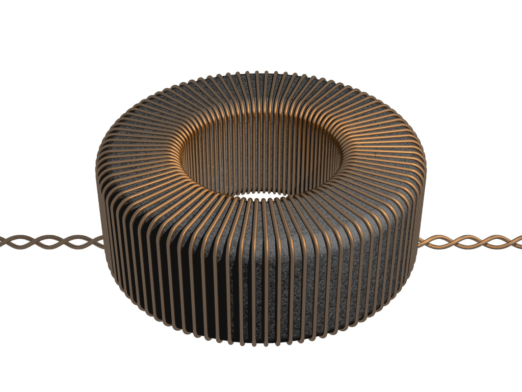
The current balun is best understood not as a transformer but as a common-mode choke — a “1:1 Guanella” in transmission-line-transformer terms. The construction is disarmingly simple: take the coax itself (or a bundled pair of wires forming a transmission line) and wind several turns through a ferrite toroid, or thread it through a string of ferrite beads. The differential transmission-line mode running inside the coax is unaffected — its equal-and-opposite currents produce equal-and-opposite flux that cancels in the core, so the core is invisible to it and the wanted signal passes with Z ≈ 0. The common-mode current, by contrast, sees the full choking inductance of the wound assembly — its flux adds in the core — and the core presents it a large series impedance. Differential mode through, common mode blocked: that is the whole trick.

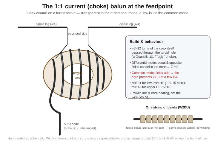
There are a few standard physical realizations, all doing the same job:

• Coax wound on a toroid. The workhorse: roughly 7–14 turns of the feed coax passed through a ferrite toroid (the 2.4-inch FT240-size core is the HF standard), potted in a weatherproof enclosure with an SO-239 on the coax side and two studs on the antenna side. This is what most commercial dipole baluns are inside.
• The “ugly balun” / air-wound choke. The same idea with no ferrite — simply 8–12 turns of the coax coiled into a tight roll. It works, but its choking impedance is lower and sharply frequency-dependent (it is a self-resonant coil), so it is a single-band expedient rather than a broadband solution. The ferrite-cored version is far better behaved across a band.
• The string-of-beads (W2DU) choke. A row of ferrite beads slid over the coax just below the feedpoint. It achieves the same series choking impedance with no winding, is light and compact, and is the classic field-portable and in-line solution. The trade is that the modest impedance of a bead string is best on the higher HF bands; getting a few kΩ down at 80 m takes a long string of the right mix.

For a single-band half-wave dipole the prescription is unambiguous: a 1:1 current balun at the feedpoint, sized for the band of use, every time. The “I’ll add one later” school pays for the omission with a year of skewed patterns, elevated receive noise, and RF in the shack. The construction details, the BOM, and the bench verification of the finished choke are in Vol 5; the broader theory of transmission-line transformers and the full family of impedance-transforming baluns and ununs (4:1, 9:1, 49:1) live in the hub’s dedicated BALUNs & UNUNs dive, which this single-band dipole volume points to rather than reproduces.

2.8 Ferrite mix, choking impedance, and power

The choke’s effectiveness lives almost entirely in the ferrite, so the mix selection deserves to be done on purpose rather than by whatever toroid is in the junk box. The figure of merit is the common-mode choking impedance Z_cm the assembly presents across the band of use — and what matters is the magnitude of that complex impedance, with a useful additional preference that it be resistive (dissipating any common-mode energy as a little heat) rather than purely reactive (which can resonate with the feedline’s common-mode impedance and actually peak the current). A practical design target is Z_cm of at least about 1 kΩ, and ideally a few kΩ (≈ 2–5 kΩ) across the operating band; that is high enough to choke the common-mode current down to insignificance against the antenna’s own feed impedance.

The two ferrite mixes that matter for HF dipole chokes are Fair-Rite type 31 and type 43, and the choice between them is a band question:

Table 1 — The two ferrite mixes that matter for HF dipole chokes are Fair-Rite type 31 and type 43, and the choice between them is a band question

Mix	Material	Best band	Why
31	MnZn ferrite, high-µ	Low–mid HF, ~1.8–15 MHz (usable across all of HF on a single core)	Highest, broadest, most resistive choking impedance through the low bands; the modern default for an all-HF dipole choke
43	NiZn, lower-µ	Upper HF and VHF, ~10–50+ MHz	Choking impedance peaks higher in frequency; the better choice for 10/6 m and VHF dipoles, and for short bead strings on the higher bands

The short version, defensible against the Fair-Rite material curves: type 31 for a choke that has to work down on 80 m and 40 m (it holds a high, usefully resistive Z_cm across the low and middle HF bands on a single FT240-31 core with about 10–14 turns), and type 43 when the band of interest is upper HF or VHF (10 m, 6 m, 2 m), where 43’s impedance peak is better placed and 31 is past its best. A great many builders standardize on a single FT240-31 choke for general HF dipole work precisely because mix 31 spans the whole HF range acceptably; the 43 choice is the deliberate one for the high-band or VHF antenna.

The constraint that surprises newcomers is that the power limit of a ferrite choke is set by core heating, not by the wire. The coax conductors carry the same differential current they always do and are nowhere near their limit; what stresses the choke is the common-mode energy and the differential flux swing dissipated in the ferrite as core loss, plus the risk of saturation if the flux density gets too high. If the common-mode impedance is too low, or the feedline is badly unbalanced (so a lot of common-mode voltage appears across the choke), the core dissipates real power, heats, and — because ferrite permeability and loss are temperature-dependent — can run away thermally and ultimately crack or de-tune. The practical consequences are that a choke should be built with enough core (a larger or stacked toroid raises the power rating), that a higher and more resistive Z_cm is also a cooler-running choke because it draws less common-mode current in the first place, and that the published power ratings of commercial baluns are heating-limited SSB/CW numbers rather than wire-current limits. Vol 1 flagged that the ends of a dipole are a high-voltage problem and the center a high-current one; the analogous truth at the feedpoint hardware is that the balun’s limit is thermal, and the build-side detail — core size, mix, turn count, and the heating-versus-power budget — is developed in Vol 5.

2.9 Feedline loss and velocity factor

Two feedline properties round out the matching picture, and both are deliberately kept at the level this volume needs — the detailed transmission-line treatment is its own subject in the hub’s feedline material.

Coax loss at HF is low but not zero. Every length of coax has a matched-line loss — the loss it exhibits when terminated in its characteristic impedance, rising with frequency and falling with cable diameter. At HF, good coax is very low-loss: a typical run of RG-8-class or LMR-400-class cable loses only a fraction of a dB across the whole feedline on the lower bands, climbing toward a dB or more only on the higher HF bands or with small cable and long runs. On top of the matched-line loss sits the additional loss under SWR introduced in Section 5 — the extra dissipation caused by the standing wave when the load is not matched. The key relationship is that additional loss under SWR scales with the matched-line loss: on a low-loss line a modest SWR adds almost nothing (the ≈ 0.05 dB of the 1.46:1 dipole), but on a lossy line — small cable, long run, or up in frequency — the same SWR can add meaningfully more, which is exactly the regime where Section 5 said a feedpoint match starts to earn its keep. The two numbers to keep straight are therefore the matched-line loss (a property of the cable, frequency, and length) and the additional loss the SWR piles on top of it (small when the matched loss is small).

Velocity factor is the ratio of the propagation speed on the line to the speed of light in free space, set by the dielectric between conductor and shield. Common values are ≈ 0.66 for solid-polyethylene coax (RG-58, RG-8, RG-213) and ≈ 0.78–0.85 for foam- or air-dielectric coax (foam-PE and gas-injected cables). For a simple dipole fed with a continuous run of coax, the velocity factor is mostly bookkeeping — it changes the physical length of cable but not the match. Where it becomes load-bearing is any place a feedline length is used as an electrical element: a quarter-wave matching transformer, a phasing line between elements, a stub, or a measured length cut to a specific electrical length. There the physical length must be the intended electrical length times the velocity factor, and getting VF wrong is a common reason a hand-cut matching section lands off-frequency. Those phasing-and-stub techniques belong to the hub’s later matching-network dives (the antenna-tuner and matching dives), not to this single-band dipole volume; the point to carry here is simply that VF exists, it is ≈ 0.66 for ordinary coax and higher for foam, and it matters the instant a length of line is doing a job other than just carrying power.

2.10 Where this volume hands off

This volume has taken ownership of the dipole feedpoint. It established the free-space 73 + j42.5 Ω and read both parts physically — the ≈ 73 Ω radiation resistance referenced to the current maximum, and the +j42.5 Ω inductive reactance that is the signature of an untrimmed-long element and that disappears when the wire is shortened by exactly the k ≈ 0.95 of Vol 1, leaving ≈ 73 Ω resistive at resonance. It traced how real ground makes that resistance oscillate with height, landing most practical dipoles between 50 and 75 Ω. It did the arithmetic that shows the 50 Ω-coax mismatch is a 1.46:1, sub-tenth-of-a-dB non-event, and said when a transformer would nonetheless matter. And it made the case that the real feedpoint problem is balance, not impedance — that common-mode current on the coax shield is the dominant real-world dipole fault, and that a 1:1 current (choke) balun at the feedpoint, mix 31 for the low bands and mix 43 for the high, sized so its choking impedance is a few kΩ and its core does not overheat, is the non-negotiable cure.

The story continues outward from the feed. Vol 3 takes the same impedance and lets frequency vary, turning the static reactance of this volume into the SWR-versus-frequency curve, the antenna’s bandwidth and Q, and develops the radiation pattern in full — the free-space donut, the ground-reflection lobing and the peak-gain-versus-height table whose impedance shadow this volume already met, NVIS at low heights, the azimuth nulls, and polarization. Vol 4 bends the clean reference into deployable shapes — folded, inverted-V, sloper, vertical dipole — each of which moves the feedpoint impedance this volume anchored. Vol 5 puts it all on a rope: the step-by-step build including winding and verifying the current balun, the trim-and-sweep tuning loop with a NanoVNA, the commercial-buy survey of feedpoint baluns, and weatherproof deployment. The broader theory of transmission-line transformers and the full balun/unun family, and the phasing-line and stub-matching techniques that lean on velocity factor, live in the hub’s dedicated matching-network dives, which this volume points to rather than duplicates.

2.11 Resources

• ARRL Antenna Book (25th+ ed.), the transmission-lines, coupling-the-line-to-the-antenna, and baluns chapters — the canonical amateur reference; reproduces the feedpoint-impedance-versus-height curves and the common-mode choke design data.
• Balanis, Antenna Theory: Analysis and Design (4th ed.) — the academic derivation of the 73 + j42.5 Ω half-wave input impedance (induced-EMF method) and the finite-length impedance behavior.
• Stutzman & Thiele, Antenna Theory and Design (3rd ed.) — complementary treatment of dipole input impedance and the effect of ground.
• Kraus, Antennas — the classic treatment of radiation resistance and the current-distribution reference for it.
• Sevick, Transmission Line Transformers (5th ed.) — the reference for current vs voltage baluns, the Guanella 1:1, and the theory the choke balun rests on.
• Fair-Rite material data sheets (mix 31, mix 43) — the defensible source for the choking-impedance-versus-frequency behavior that drives the mix-by-band selection in §8.