The Canonical Half-Wave Dipole

---

1.1 About this volume

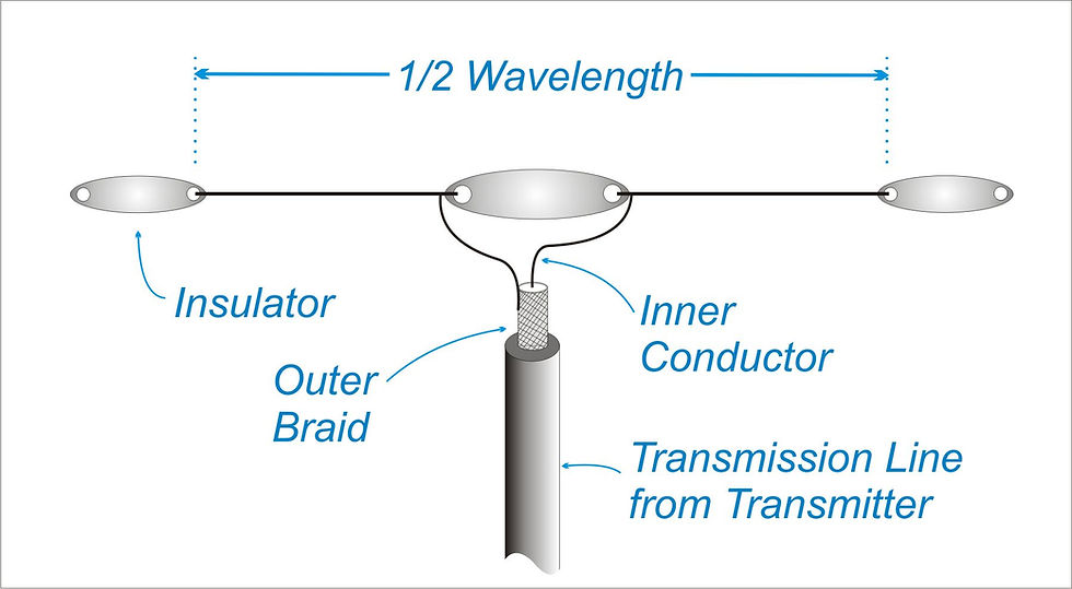
The half-wave dipole is the antenna every other antenna is compared to. Decibels referenced to a dipole carry the suffix dBd, and the conversion dBi = dBd + 2.15 is the linguistic glue between free-space gain and what the rest of the antenna literature actually quotes. If you understand a dipole — the standing wave that lives on it, why the moving charge on it radiates, how long to cut it and why that length is a few percent shorter than a textbook half-wavelength — you understand the spine of nearly every practical antenna in this series. A Yagi’s driven element is a dipole; a quad’s driven loop is a folded dipole bent into a square; a log-periodic is a graded array of dipoles; even a vertical monopole is half of one working against its image. The geometry here is load-bearing for everything downstream.

This first volume deliberately stays inside the fundamentals of the canonical center-fed half-wave element: the standing-wave picture, the radiation mechanism, the end-effect, the cut-to-length arithmetic, and the gain reference. The companion volumes carry the rest of the single-band dipole story and are forward-referenced where they belong rather than pre-empted here. Feedpoint impedance, the 73 + j42 Ω free-space figure, and the 1:1 current balun that belongs at every dipole’s feedpoint are the subject of Vol 2 — Feedpoint impedance and matching. The radiation pattern (the free-space donut, the ground-reflection lobing that lifts a horizontal dipole toward ~7.8 dBi at half-wave height, NVIS, and the SWR-versus-frequency curve) is Vol 3 — Radiation pattern, ground effect and SWR. The mechanical and topological variants that still belong to the single-band family — folded, inverted-V, sloper, vertical dipole — are Vol 4 — Variants. The hands-on build, tuning with a NanoVNA, and the commercial-buy survey are Vol 5 — DIY build, tuning, buys and deployment. The multi-band relatives (off-center-fed, fan, trap, doublet, G5RV, ZS6BKW, linked) are a different problem and live in their own dive entirely.

What this volume nails down — the cosine current distribution, the k ≈ 0.95 trim factor and its dependence on the element’s length-to-diameter ratio, the derivation of 468/f_MHz, and the 2.15 dBi directivity — are the numbers the rest of the hub leans on. Get them right once, here, and the later volumes inherit a clean foundation.

1.2 Standing waves on a half-wave element

A half-wave conductor fed at its center is a resonator, and the resonant condition is a standing wave whose geometry is fixed by the boundary conditions at the two open ends. The ends are open circuits: no current can flow past a wire tip into thin air, so the current must go to zero there. The center is the driven point. The only sinusoidal current distribution that satisfies zero at both ends on an element one half-wavelength long is a single half-cycle of a cosine, measured from the center. Writing z for position along the element with z = 0 at the feedpoint and β = 2π/λ the phase constant, the resonant current and voltage envelopes are

I(z) ≈ I₀ · cos(βz) and V(z) ≈ V₀ · sin(βz),

valid for −λ/4 ≤ z ≤ +λ/4. The current is maximum at the center and falls to zero at each end; the voltage is the spatial quadrature partner — zero at the center and rising to a maximum at each end. They are 90° apart in space and (for the lossless resonant case) 90° apart in time, which is exactly the relationship a quarter-wave-long open-circuited transmission-line stub presents transformed to its driven end. A dipole, electrically, is a pair of such stubs spread open into radiating arms.

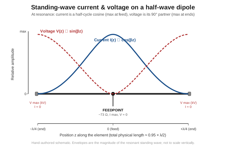
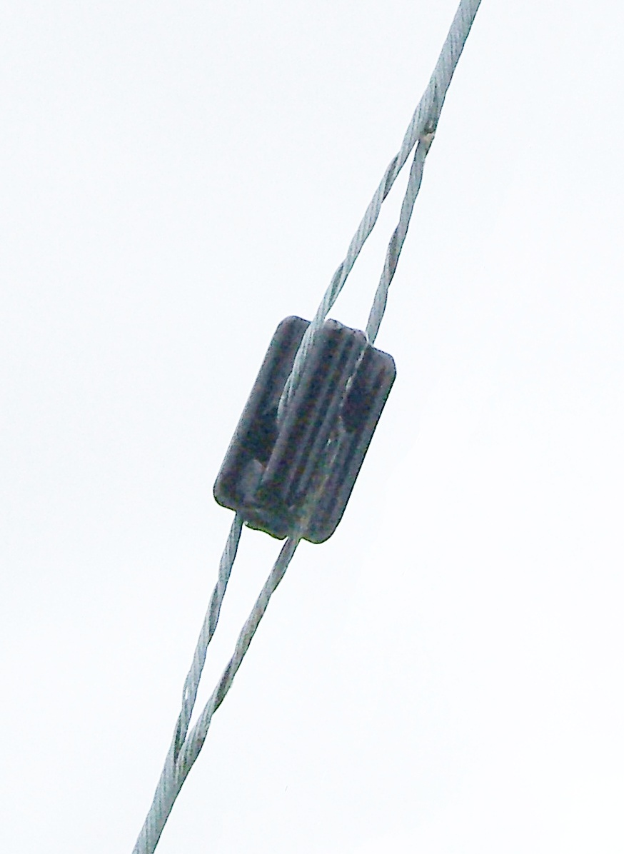
The consequences of this picture are not decorative; they dictate where the antenna’s hardware stress lives and how you feed it. Because the peak current is what radiates (the next section makes that precise), the center of a dipole is where most of the radiation originates, not the ends — a fact that runs counter to the intuition that “the action is at the tips.” The near-field structure, the common-mode behavior of the feedline, and the right feeding strategy are therefore all centered on the geometric center. Two practical rules fall straight out. First, the feedpoint wants conductivity: it sits at a current maximum and a low voltage (~73 Ω at resonance, derived in Vol 2), so any resistance there — a corroded joint, an undersized lug, a lossy connector — dissipates real power as I²R heat at the exact point the current is largest. Second, the ends want dielectric strength: they sit at a voltage maximum, and at legal-limit power the standing-wave voltage at the tips of a thin-wire dipole runs into the low kilovolts. That is why dipole ends terminate in ceramic or high-grade polymer insulators rather than whatever plastic is in the junk box — the insulator is a high-voltage RF component, not a piece of string-tie hardware.

The standing wave also explains why the antenna is narrowband in the way it is. The cosine current distribution is the natural mode of the structure only at and very near the frequency where the element is a half-wavelength. Move off that frequency and the boundary conditions can no longer be satisfied by a pure resonant standing wave with zero reactance — the element looks slightly inductive above resonance and slightly capacitive below it. The bandwidth over which the resulting reactance stays small enough to feed comfortably, and the SWR curve that traces it, are the subject of Vol 3; for now the key idea is that the clean cosine distribution is the resonant condition, and everything off-resonance is a perturbation of it.

1.3 Why a half-wave dipole radiates

It is worth being precise about the physical mechanism, because the most common mental model — “the RF wave travels out to the open end, reflects, and bounces back and forth” — is a circuit-theory description that is mathematically serviceable but physically misleading. The standing wave is real, but it is not why the antenna radiates; it is the steady-state current distribution that results once you drive the structure at resonance. Radiation comes from a deeper and simpler fact of electromagnetism: accelerating charge radiates. A charge moving at constant velocity does not; a charge whose velocity is changing — equivalently, a conductor carrying a time-varying current, dI/dt ≠ 0 — launches a field that detaches from the conductor and propagates away as a wave. A half-wave dipole, carrying a sinusoidal current that reverses 2f times a second, is a structure optimized to accelerate as much charge as possible in as nearly-uniform a phase as a simple wire geometry allows.

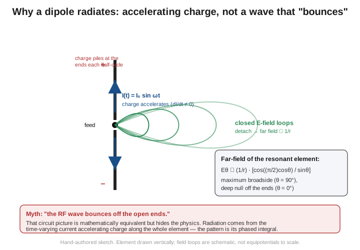
The far field follows from integrating that current distribution against the geometric phase delay across the antenna’s length. Each infinitesimal length dz of the element is a Hertzian current element radiating its own spherical wavelet; the wavelets from different parts of the antenna arrive at a distant observer with phase differences set by the path-length difference, and they sum. Carrying the integral through for the cos(βz) distribution of a half-wave element gives the classic closed-form pattern factor

E_θ ∝ (1/r) · [ cos((π/2)·cos θ) / sin θ ],

where θ is measured from the wire axis. This is maximum broadside to the wire (θ = 90°) and has a deep null off each end (θ → 0), which is the figure-8 azimuth pattern and the elevation circle that together make the free-space “donut.” The full pattern, its lobing over ground, and the polarization consequences are detailed in Vol 3; the point to carry from this volume is that the pattern is the phased integral of the current distribution, not the result of anything bouncing.

The reason the misconception matters is that it predicts the wrong things. If radiation came from energy sloshing off the ends, you would expect the ends to be the radiating parts and the center to be quiet — exactly backwards. The accelerating-charge picture predicts the opposite and correctly: the current maximum at the center is where the most charge is being accelerated, so the center dominates the radiation, and any modification that flattens and smooths the current distribution (a fat element, a folded dipole) broadens the bandwidth at little cost to gain, while any modification that crowds current toward the high-impedance ends (heavy end-loading, a top hat on a shortened element) trades gain away. The clean, near-sinusoidal current distribution of the full-size half-wave element is precisely why it sets the gain reference in §7.

1.4 The end-effect and velocity factor on the wire

A wire dipole cut for resonance is consistently a few percent shorter than a free-space half-wavelength, and the deep dive on antenna behavior collapses an awful lot of real physics into the offhand “cut it to 95%.” Two related effects produce that shortening, and it is worth separating them because they scale differently.

The first and dominant one is the end-effect. The wire does not end in an abrupt electrical discontinuity; the tips, the end insulators, and the doubled-back wire of the termination loop all add a small shunt capacitance to the high-voltage ends of the element. That capacitance stores reactive energy and is electrically equivalent to a short additional length of wire — so the physical wire needed to reach resonance is shorter than the electrical half-wavelength by the amount the end capacitance “adds back.” The end-effect is concentrated at the tips, where the voltage (and hence the electric field into the surrounding dielectric) is highest, which is exactly why it depends on what is at the ends: bare wire over open air shortens least, a wire whose ends are wrapped through bulky insulators or run close to a metal mast shortens more.

The second effect is the slightly reduced velocity of propagation along the conductor relative to free space. A real wire has finite diameter and finite conductivity, and the guided wave travels marginally slower than c; an insulating jacket on the wire slows it further still, because part of the field now lives in the jacket’s dielectric rather than in air. Slower propagation means the physical length corresponding to a given electrical length is shorter. For bare HF wire this is a small contributor next to the end-effect; for PVC- or polyethylene-jacketed wire it becomes significant, and insulated-wire dipoles routinely come out 2–4% shorter still than the bare-wire number.

Both effects are folded into a single dimensionless trim factor k, defined by

L_physical = k · (λ/2),

with k a function primarily of the element’s length-to-diameter ratio (ℓ/d). A thin element — high ℓ/d — has a small end region relative to its length and a k close to 0.96–0.97; a fat element — low ℓ/d, such as tubing — has proportionally more end capacitance and a smaller k. The dependence is monotonic and well documented in the antenna literature (the ARRL Antenna Book reproduces the classic k-versus-ℓ/d curve, and Balanis derives the underlying length correction):

Table 1 — with k a function primarily of the element's length-to-diameter ratio (ℓ/d). A thin element — high ℓ/d — has a small end region relative to its length and a k close to 0.96–0.97; a fat element — low ℓ/d, such as tubing — has proportionally more end capacitance and a smaller k. The dependence is monotonic and well documented in the antenna literature (the ARRL Antenna Book reproduces the classic k-versus-ℓ/d curve, and Balanis derives the underlying length correction)

Element	length / diameter (ℓ/d)	k (approx.)	Notes
#18 thin wire	25,000+	0.96	Minimal end-effect; the curve’s “thin” asymptote
#14 / #12 antenna wire	5,000–15,000	0.95	The standard HF dipole; 468/f_MHz (feet) assumes this
#10 stranded	3,000–6,000	0.94	Slight fattening trim
3/16″ tubing	800–1,500	0.93	Fat element — upper HF (≈10–15 m)
1/2″ tubing	80–250	0.92	VHF dipoles (6 m, 2 m) from rod or tubing
Insulated (PE/PVC) #14	5,000–15,000	0.92–0.94	Jacket lowers velocity factor; cut 2–4% shorter than bare

The thin-wire HF case — k ≈ 0.95 — is the one the canonical cut-to-length formula assumes, and the next section derives that formula from it. The fat-element cases matter because a 6 m or 2 m dipole built from rod or tubing genuinely resonates short of the thin-wire number, and a VHF builder who cuts to 468/f will find the antenna resonant low and have to file the element shorter. The general guidance that flows from the whole table is to cut long and trim: the trim factor is a starting estimate, the real number depends on your exact wire, insulators, and surroundings, and a pair of side cutters only ever makes a wire shorter. The mechanics of that trim-and-sweep loop are in Vol 5.

1.5 The 468/f rule, derived

The number every wire-antenna builder has memorized is L_feet = 468 / f_MHz for the total length of a thin-wire half-wave dipole. It is worth deriving rather than memorizing, both so you can see exactly which assumptions are baked into it and so you can correct it when those assumptions break.

Start from the speed of light expressed in the builder’s units. In feet per second, c ≈ 9.836 × 10⁸ ft/s, so a free-space wavelength is

λ_feet = 983.6 / f_MHz ≈ 984 / f_MHz.

A free-space half-wavelength is therefore

(λ/2)_feet = 492 / f_MHz

— this is the length a half-wave element would be if the wire behaved exactly like free space, with no end-effect and no velocity reduction. Now apply the thin-wire trim factor from §4, k ≈ 0.95:

L_feet = 0.95 × 492 / f_MHz = 467.4 / f_MHz ≈ 468 / f_MHz.

That is the whole derivation. The famous 468 is nothing more than 0.95 × 492 = 467.4, rounded to the convenient integer 468 that the literature has used by convention ever since, and the per-leg length is half of it, 234 / f_MHz. The metric form follows identically from c ≈ 3.00 × 10⁸ m/s: λ_m = 300/f_MHz, the free-space half-wave is 150/f_MHz, and with the same k ≈ 0.95,

L_m ≈ 142.5 / f_MHz (per leg ≈ 71.3 / f_MHz),

which is also exactly 468 / f_MHz feet converted at 0.3048 m/ft (468 ft → 142.65 m), so the two formulas are the same statement in different units. Some references quote 143/f for the metric constant; the one-part-in-300 difference is rounding noise well below the trim tolerance.

The value of the derivation is that it makes the formula’s failure modes obvious, because they are exactly the cases where k = 0.95 is wrong:

• Very thin wire (#18 and finer, or a single-strand stealth wire) has k closer to 0.96, so 468/f cuts it slightly short; around 472/f is the better starting estimate for hairline wire.
• Fat elements — tubing or rod on 6 m, 2 m, and up — have k of 0.92–0.94, so 468/f cuts them long and they resonate low. For VHF tubing dipoles, design from a k-versus-ℓ/d curve (or a NEC model) rather than the thin-wire constant; 460/f or shorter is typical.
• Insulated wire carries part of its field in the jacket dielectric, dropping the velocity factor and pulling resonance down; expect to cut a PE-jacketed #14 dipole 2–4% shorter than 468/f.
• Proximity to ground, metal, or foliage detunes the element through capacitive coupling and induced currents, almost always lowering the resonant frequency; a dipole strung close to a metal gutter or a wet tree will not land where 468/f predicts.

In every one of these cases the formula is a first cut, not a final dimension — which is the entire reason the build procedure in Vol 5 is “cut to 468/f plus a percent, hoist, sweep, trim.” The formula gets you within trimming range; the analyzer gets you onto frequency.

1.6 Half-wave length table — every band of interest

The table below applies the thin-wire formula directly: total length = 468 / f_MHz (feet) = 142.6 / f_MHz (metres), with each leg half of that. These are the lengths to cut to as a starting point for #14 wire, then trim onto frequency with an analyzer per Vol 5. The design frequencies chosen are sensible band-centres for a general-purpose dipole; pick your own design frequency to favour the CW or phone end and recompute — the formula scales linearly, so a 1% change in frequency is a 1% change in every length.

Table 2 — 6. Half-wave length table — every band of interest

Band	Design freq (MHz)	Total length (ft)	Total length (m)	Each leg (ft)	Each leg (m)
160 m	1.900	246.3	75.08	123.2	37.54
80 m	3.650	128.2	39.08	64.11	19.54
60 m	5.358	87.35	26.62	43.67	13.31
40 m	7.150	65.45	19.95	32.73	9.98
30 m	10.125	46.22	14.09	23.11	7.04
20 m	14.175	33.02	10.06	16.51	5.03
17 m	18.118	25.83	7.873	12.92	3.94
15 m	21.225	22.05	6.721	11.02	3.36
12 m	24.940	18.77	5.720	9.38	2.86
10 m	28.500	16.42	5.005	8.21	2.50
6 m	50.250	9.31	2.839	4.66	1.42
2 m	146.00	3.21	0.977	1.60	0.489
70 cm	446.00	1.05	0.320	0.525	0.160

Two cautions on reading the table. First, the 160 m and 80 m entries are physically large — a full-size 160 m dipole is roughly 75 m of wire end-to-end, and 80 m is nearly 40 m — so on a typical lot the install geometry, not the antenna theory, is the limiting factor; the variants and deployment tricks in Vol 4 (the inverted-V’s single-support footprint especially) are where that problem gets managed. Second, the 2 m and 70 cm rows are nominal only. The thin-wire 468/f formula assumes the HF k ≈ 0.95, but a VHF/UHF dipole is almost always built from rod or tubing whose ℓ/d is far lower, so the real k is 0.92–0.94 and the resonant element is shorter than the table says. Treat the VHF figures as a place to start filing from, and expect to design those from a fat-element correction or a model as discussed in §4–5. The single most common new-builder error the table guards against is a factor-of-two slip — cutting a “40 m” dipole to the 20 m length (or vice versa) — whose unmistakable symptom is an antenna whose lowest SWR lands at twice (or half) the intended frequency. Read the band off the design-frequency column, not from habit.

1.7 The 2.15 dBi reference — defining the dipole as 0 dBd

The half-wave dipole is not just an antenna; it is the agreed-upon yardstick, and that role rests on a single number. A lossless, infinitely-thin half-wave dipole in free space has a directivity of 1.64 as a linear power ratio, which in decibels relative to an isotropic radiator is

10 · log₁₀(1.64) = 2.15 dBi.

That figure is the formal definition of the dBd scale: a gain of “0 dBd” means “the same gain as a half-wave dipole,” so by construction dBi = dBd + 2.15. When a Yagi is advertised at “6 dBd,” it means 6 dB better than a dipole in the same situation, i.e. 8.15 dBi; the two scales differ by exactly the dipole’s own 2.15 dB head start over the isotropic fiction. (For comparison, the infinitesimal Hertzian dipole’s directivity is 1.5, or 1.76 dBi — the half-wave element’s slightly higher 1.64 comes from its current taper, which concentrates the pattern marginally more toward broadside.)

Two qualifications keep this honest. First, the 2.15 dBi is a directivity — it describes how the radiated power is distributed in angle, not how much of the input power gets radiated at all. For a full-size copper dipole the radiation efficiency is essentially 100% (the radiation resistance dwarfs the wire’s ohmic resistance), so directivity and gain are interchangeable to a small fraction of a dB; the distinction only bites for shortened or heavily loaded elements where ohmic and loading losses eat into efficiency, which is not the canonical case this volume treats. Second — and this is the qualification that trips up every gain comparison — the 2.15 dBi is a free-space number. The instant you put the dipole over real ground at a finite height, ground reflection rearranges the pattern into lobes and the peak gain in the favoured direction rises well above 2.15 dBi (toward roughly 7.8 dBi at a height of half a wavelength), while the gain at other angles falls below it. A “dipole has 2.15 dBi of gain” statement is therefore only unambiguous in free space; over ground the right answer is “it depends on height,” and that height-dependent lobing is worked out in full in Vol 3. The free-space 2.15 dBi is the number that defines the reference; the over-ground numbers are what you actually transmit with.

1.8 Resonant, off-resonant, and what “resonant” buys you

“Resonant” has a precise meaning for a dipole, and it is narrower than “works well.” A half-wave element is resonant at the frequency where its feedpoint reactance is zero — where the leftover inductive reactance above resonance and capacitive reactance below it cross through X = 0 and the feedpoint looks purely resistive. At that frequency the cosine current distribution of §2 is the natural mode of the structure, the feedpoint presents its resistive ~73 Ω (free space; less over ground), and the antenna can be fed on coax with no matching network beyond the current balun. Resonance is a property of the element’s electrical length, set by the trim factor and the cut; it is what the whole §4–6 length apparatus exists to deliver.

The point worth internalising is that resonance is a feeding convenience, not a radiating requirement. A dipole an appreciable fraction off its resonant frequency still radiates perfectly well — the current distribution is only mildly perturbed from the resonant cosine, the radiation efficiency and the pattern barely move over a few percent of bandwidth, and the antenna will happily put your power into the far field. What changes off-resonance is the feedpoint: the reactance is no longer zero, so the feedpoint impedance walks off into complex territory (inductive above resonance, capacitive below), the SWR on a 50 Ω line climbs, and the reflected energy has to be managed. Near resonance that management is trivial — a clean dipole on coax holds an acceptable SWR across a useful band, the bandwidth of which is set by the element’s Q and is mapped out in Vol 3. Push further off-resonance — using a 40 m dipole on 15 m, say — and the reactance grows large enough that you need a transmatch at the shack end to present the radio a 50 Ω load, even though the antenna itself is still radiating. The distinction between the antenna radiates and the feedline/tuner is happy is the single most clarifying idea in practical dipole work, and the matching machinery that bridges the two — balun, line, tuner — is the entire subject of Vol 2.

This is also why the standard build is “cut for resonance at your favourite part of the band.” You are not chasing resonance because the antenna refuses to radiate elsewhere; you are chasing it because a resonant dipole is the one operating point where the feed problem disappears and a length of coax and a 1:1 balun are the whole matching system. Everything else costs you a tuner, some feedline loss, or both.

1.9 Where this volume hands off

This volume has fixed the geometry and the physics of the canonical half-wave element: the standing-wave current and voltage distributions and what they demand of the feedpoint and the ends; the accelerating-charge radiation mechanism and the broadside far-field pattern that integrates out of it; the end-effect and velocity-factor shortening rolled into the trim factor k; the derivation of 468/f_MHz and its metric twin and the cases where they need correcting; the band-by-band length table; the 2.15 dBi directivity that makes the dipole the 0 dBd reference; and the precise meaning of resonance as a zero-reactance feeding convenience rather than a radiating requirement.

The single-band dipole story continues from here. Vol 2 takes the feedpoint seriously — the 73 + j42 Ω free-space figure, the height-dependent impedance over real ground, the 50 Ω-coax mismatch and why it is harmless, and the 1:1 current balun that belongs at every dipole feedpoint. Vol 3 develops the radiation pattern in full — the free-space donut, the ground-reflection lobing and peak-gain-versus-height table, NVIS at low heights, the azimuth nulls, polarization, and the SWR-versus-frequency curve and bandwidth. Vol 4 covers the variants that bend this clean reference into more deployable shapes — folded, inverted-V, sloper, and vertical dipole. Vol 5 puts it all on a rope: a step-by-step DIY build, the trim-and-sweep tuning loop with a NanoVNA, the commercial-buy survey, and weatherproof deployment.

1.10 Resources

• ARRL Antenna Book (25th+ ed.), the dipole and inverted-V chapter — the canonical amateur reference; reproduces the k-versus-ℓ/d trim-factor curve and the 468/f derivation.
• Balanis, Antenna Theory: Analysis and Design (4th ed.) — the academic reference for the half-wave dipole far-field derivation, the 1.64 directivity, and the finite-length length-correction.
• Stutzman & Thiele, Antenna Theory and Design (3rd ed.) — complementary treatment of the dipole current distribution and pattern integral.
• Kraus, Antennas — the classic derivation of radiation from a current element and the dipole pattern factor.