Yagi-Uda Antennas · Volume 2
Boom Length, Gain, and Pattern
The diminishing-returns gain curve corrected against real NEC-modeled data, front-to-back ratio and side-lobe suppression, the gain/bandwidth/F-B triangle quantified, half-power beamwidth and the aiming consequence, and stacking as the alternative to a longer boom
2.1 About this volume
Vol 1 established the parasitic-array mechanism — how a reflector and a string of directors, each tuned slightly off the driven element’s resonance, re-radiate the driven element’s field with a phase relationship that adds constructively forward and destructively aft, and how the mutual impedance between closely-spaced elements sets the current each one actually carries. This volume takes that mechanism as given and asks the question every Yagi designer and buyer actually cares about: for a given amount of boom, how much forward gain do you get, in what shape, and at what cost to everything else the antenna does? Those “everything else” items — front-to-back ratio, side-lobe level, half-power beamwidth, and bandwidth — are not independent knobs. They are four faces of the same current distribution along the same boom, and pushing on one moves the others, usually against you.
The chapter this volume replaces carried a specific, quotable error: a “gain (dBd) ≈ 10·log₁₀(boom in λ) + 7” rule of thumb, presented as valid “from 2-element to 20-element designs,” checked against the very gain table sitting two paragraphs below it. It is not valid across that range, and the disagreement is not a rounding issue — recomputing the formula against the table’s own numbers turns up a sign-changing error: at the 2-element end the formula predicts negative gain relative to a dipole, which is a physical impossibility for an antenna that has a reflector and driven element adding constructively by construction. Section 2 works out why a single log-law formula cannot span the whole range, states the domain where a corrected version of it actually holds (checked against independently published NEC-modeled data, not just against the seed’s own numbers), and shows the physical reason the short-boom end behaves completely differently. Sections 3–4 take up front-to-back ratio and side-lobe level — what they cost, and who actually needs to pay for suppressing them past the amateur default. Section 5 renders the classic “pick two of three” gain/bandwidth/F-B tradeoff as a real figure with real numbers rather than the ASCII triangle the seed chapter drew. Section 6 gives the beamwidth-by-element-count table its aiming consequence and hands the rotator-and-accuracy discussion to Vol 4, which owns installation and pointing hardware. Section 7 closes with stacking — the alternative to a longer boom that most operators reach for once a single Yagi’s boom has grown past what a tower or rotator will comfortably carry.
One more housekeeping note earns its place here because it bears directly on how much confidence to put in any single number in this volume: the seed chapter actually offered three separate accounts of the same gain-vs-length relationship — the per-director incremental-gain list, a “3 dB per doubling” bandwidth-doubling table, and the main gain-vs-boom table — and, checked against each other, they do not agree. That is worked through in §2.3, because it is exactly the kind of internal inconsistency a reader building a Yagi from a single source would never catch without doing the arithmetic, and it is the clearest illustration of why this volume treats every boom-length/gain number as provisional until it is checked against an independent source or against the antenna’s own physics.
2.2 Boom length vs gain — the diminishing-returns curve, corrected
2.2.1 The claim, and why it cannot be right as stated
The migrated chapter’s rule of thumb was gain (dBd) ≈ 10·log₁₀(L/λ) + 7, claimed to hold “from 2-element (boom ~0.15λ) to 20-element (boom ~6λ) designs.” Running that formula against the chapter’s own gain table turns up the following:
Table 1 — The migrated chapter's rule of thumb was gain (dBd) ≈ 10·log₁₀(L/λ) + 7, claimed to hold "from 2-element (boom ~0.15λ) to 20-element (boom ~6λ) designs." Running that formula against the chapter's own gain table turns up the following
| Elements | Boom (λ) | Formula (dBd) | Chapter’s table (dBd) | Delta |
|---|---|---|---|---|
| 2 | 0.15 | −1.24 | 4.5 | −5.74 |
| 3 | 0.40 | 3.02 | 6.5 | −3.48 |
| 5 | 1.00 | 7.00 | 9.0 | −2.00 |
| 9 | 2.20 | 10.42 | 11.2 | −0.78 |
| 15 | 4.00 | 13.02 | 13.0 | +0.02 |
| 28 | 8.00 | 16.03 | 15.0 | +1.03 |
The delta is not just large at the short-boom end — it changes sign across the table, from a formula that badly underestimates gain at 2–5 elements to one that mildly overestimates it at 28. A formula whose error flips sign as you scan its own claimed domain is not a slightly-imprecise approximation; it is being asked to do something a single log-linear curve cannot do. And the 2-element row is worse than “imprecise”: 10·log₁₀(0.15) + 7 = −1.24 dBd says a 2-element Yagi radiates less forward gain than a bare dipole. That is not physically possible for this antenna. Vol 1 established that a reflector re-radiates the driven element’s field with a phase delay that adds constructively in the forward direction and destructively to the rear — by the very mechanism that makes it a “reflector” and not just an inert rod, the pair has to gain over a lone dipole, and every measured or NEC-modeled 2-element Yagi in the literature shows a positive gain figure, typically in the 4–7 dBd range depending on spacing and tuning. A rule that predicts the opposite sign for the shortest, most common beam element-count in amateur use is not a rule that “works well” down to two elements; it fails there outright, and the seed chapter’s claim to the contrary does not survive contact with its own numbers.
2.2.2 Two regimes, one physical reason
The fix is not a different constant — it is recognizing that “gain as a function of boom length” describes two genuinely different physical regimes, and a single formula built to fit one regime will misbehave in the other.
Below roughly 1λ of boom (in practice, 2 to about 4–5 elements), the antenna’s gain is dominated by strong near-field mutual coupling between a small number of tightly-spaced elements — exactly the phase-and-spacing mechanism Vol 1 derived in detail. The seed chapter’s own per-director incremental-gain list makes the point without needing outside data: it credits the first director alone with +1.5 to +2.0 dB of gain, contributed by a single element sitting roughly 0.15–0.2λ from the driven element — a fraction of a wavelength of boom buying nearly two full decibels. That is not an aperture antenna accumulating gain the way a phased array accumulates gain with more radiating length; it is two or three elements exchanging energy through their mutual impedance at close range, and the “boom length” number for that regime is almost incidental — what matters is the number of elements and their individual spacing and tuning, not the aggregate length they happen to occupy. A log-of-length model has no way to see this, because the model’s entire premise is that length is the free variable driving gain; in the 2–4-element regime, length is nearly fixed by the coupling geometry and gain instead tracks element count.
Above roughly 1–2λ of boom (in practice, from about 5 elements up through the long EME-class designs), the antenna transitions into something closer to a traveling-wave, end-fire aperture — the physical picture Hermann Ehrenspeck and Walter Poehler formalized in their 1959 analysis “A New Method for Obtaining Maximum Gain from Yagi Antennas” (IRE Transactions on Antennas and Propagation, October 1959), which modeled a long director string as supporting a surface wave traveling along the array and showed that, for a given phase velocity of that wave, gain becomes a systematic function of the array’s physical length. In this regime a log-linear approximation of the form gain (dBd) ≈ 10·log₁₀(L/λ) + C is a genuinely reasonable description — not because the physics is logarithmic in any fundamental sense, but because an end-fire aperture’s directivity grows with length in a way that a log-law, fit over a bounded range, approximates well.
2.2.3 The seed’s own three accounts disagree with each other
Before settling on a corrected formula it is worth actually doing the arithmetic on the seed chapter’s three separate presentations of this same relationship, because they do not cross-check, and a reader who only skimmed the prose would not notice. The per-director incremental list (§3.3 of the migrated chapter) gives each added director’s gain contribution as a range; chaining the upper end of every increment starting from the main table’s own 2-element figure (4.5 dBd) lands exactly on the table’s 3-element figure (6.5 dBd, +2.0 dB for the first director) — but then overshoots the table’s 4-element figure by 0.2 dB (7.7 dBd chained vs 7.5 dBd tabulated), before falling increasingly short from 5 elements on: 8.5 vs a tabulated 9.0 (−0.5 dB), widening to roughly −0.7 to −0.9 dB by 6 through 9 elements. So the two internal accounts do not just disagree by a fixed offset — they cross over, matching exactly at one element count, overshooting at the next, and undershooting by nearly a full dB two elements later. Two tables in the same source, both purporting to describe the same antenna family, cannot even agree on the direction of their own disagreement.
The “3 dB per doubling” claim (§4.1 of the migrated chapter) fares worse. Its own worked table lists five boom-length steps and the gain each adds; only one of those five steps is an actual doubling of boom length (15-element, 4.0λ, to 28-element, 8.0λ), and that literal doubling adds 2.0 dB, not the 3 dB the section’s own header claims. The other four steps are not doublings at all (ratios of 1.4× to 2.5×) and their added gain — 2.5, 1.3, 1.6, and 1.1 dB respectively — is consistently below the 10·log₁₀ prediction for their respective ratios, which would call for 3.98, 2.04, 2.43, and 1.55 dB. Every single row of the seed’s own “3 dB per doubling” table under-delivers against both a literal doubling and against the log-law it is nominally illustrating. None of this means “3 dB per doubling” is a useless rule of thumb — it is a fine order-of-magnitude gut-check for a first-pass design conversation — but it is not what the seed’s own numbers show, and a table that contradicts its own section header is a specific, checkable defect worth naming rather than silently repeating.
The lesson generalizes past this one migrated chapter: three internally-inconsistent accounts of “how gain scales with boom length” made it into a single source, and the inconsistency is only visible if you actually run the numbers against each other rather than reading the prose in isolation. Every gain-versus-length number in the rest of this section has been checked against an outside, independently-modeled source for exactly this reason.
2.2.4 A corrected formula, with an honest domain
Cross-checking against real NEC-modeled data rather than against the seed chapter’s own arithmetic gives a formula that actually holds. L. B. Cebik (W4RNL) published a comparison of DL6WU-tradition long-Yagi designs at 432 MHz (“70-CM Yagi Stacks Part 1: 10- to 40-Element DL6WU Examples”) with the following NEC-modeled free-space gain figures:
Table 2 — Cross-checking against real NEC-modeled data rather than against the seed chapter's own arithmetic gives a formula that actually holds. L. B. Cebik (W4RNL) published a comparison of DL6WU-tradition long-Yagi designs at 432 MHz ("70-CM Yagi Stacks Part 1: 10- to 40-Element DL6WU Examples") with the following NEC-modeled free-space gain figures
| Elements | Boom (λ) | Gain (dBi) | Gain (dBd) |
|---|---|---|---|
| 13 | 3.225 | 15.28 | 13.13 |
| 19 | 5.615 | 17.21 | 15.06 |
| 28 | 9.215 | 18.92 | 16.77 |
| 34 | 11.615 | 19.75 | 17.60 |
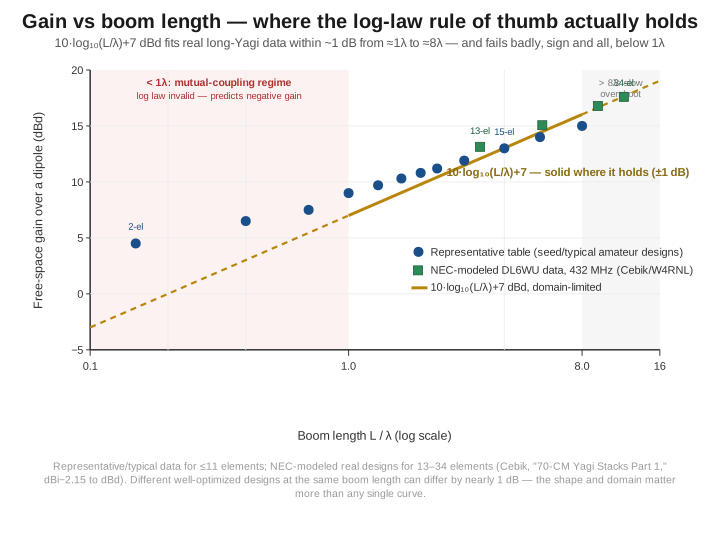
Fitting gain (dBd) ≈ 10·log₁₀(L/λ) + 7 against these four real, independently-modeled points gives predictions of 12.09, 14.49, 16.64, and 17.65 dBd — errors of −1.04, −0.57, −0.13, and +0.05 dB. That is a genuinely good fit, tightening as boom length grows, across a boom range from 3.2λ to 11.6λ (roughly 13 to 34 elements). The same formula, over the same physical mechanism, is doing real work here — which is exactly why it is worth keeping rather than discarding outright. The corrected statement is therefore a bounded one: gain (dBd) ≈ 10·log₁₀(L/λ) + 7 is a reasonable approximation from roughly 1λ to 8–10λ of boom (very roughly 5 to 30 elements), typically accurate to within about 1 dB against independently NEC-modeled long-Yagi data, and it should not be extrapolated below about 1λ, where it fails outright.
Two further honesty notes belong here rather than in a footnote. First, back-solving the constant C from each of the four Cebik data points individually (rather than fitting a single value across all of them) gives 10.19, 9.72, 9.28, and 9.10 dBi as boom length runs from 3.2λ to 11.6λ — a slow downward drift of about a decibel over that span, consistent with the seed chapter’s own qualitative observation that “the diminishing-returns curve gets steeper at longer boom lengths.” A fixed-constant log-law is a good approximation over any bounded window of this range, but the true curve flattens a little faster than a single global constant admits once boom length pushes past about 8λ — which is also where the seed table’s own 28-element figure (15.0 dBd, 17.15 dBi) undercuts Cebik’s own 25-element model at essentially the same boom length (8.015λ, 18.45 dBi / 16.30 dBd) by about 1.3 dB, itself a symptom of the same effect working in the opposite direction: at this extreme length, different well-optimized real designs can disagree by more than the fixed-C formula’s own already-small error band. Second, a widely-repeated observation from the CB-antenna modeling community (a compilation of “over 40 NEC and AN-SOF modeled antennas” published at cb-antennas.com) is that “differences between good designs are less than 1 dB for a given boom length” — which is the honest ceiling on how precisely any single formula or table should be trusted to predict a specific real antenna’s gain. The value of this section’s corrected formula is in its domain and its shape, not in a claim to third-decimal-place accuracy.
Below about 1λ, do not use the formula at all — use tabulated, per-design figures instead, understanding that the physics there is mutual-coupling-dominated (§2.2) and that the seed chapter’s own 2- through 4-element gain figures (4.5, 6.5, and 7.5 dBd respectively) are representative of typical, reasonably-optimized short designs rather than a value derivable from boom length alone. This is precisely the domain where Vol 1’s per-director mutual-impedance treatment, not an aperture-gain formula, is the right tool.
2.2.5 A gain-vs-boom table with its regimes labeled
Putting the representative short-boom figures and the NEC-modeled long-boom figures side by side, with the domain of the corrected formula marked explicitly:
Table 3 — Putting the representative short-boom figures and the NEC-modeled long-boom figures side by side, with the domain of the corrected formula marked explicitly
| Elements | Boom (λ) | Gain (dBd) | Gain (dBi) | Regime |
|---|---|---|---|---|
| 2 | 0.15 | ~4.5 | ~6.65 | mutual coupling — formula invalid |
| 3 | 0.40 | ~6.5 | ~8.65 | mutual coupling — formula invalid |
| 5 | 1.0 | ~9.0 | ~11.15 | transition — formula runs ~2 dB low |
| 9 | 2.2 | ~11.2 | ~13.35 | log-law domain — formula runs ~0.8 dB low |
| 13 | 3.225 | 13.13 | 15.28 | log-law domain, NEC-modeled (Cebik/DL6WU) |
| 19 | 5.615 | 15.06 | 17.21 | log-law domain, NEC-modeled |
| 28 | 9.215 | 16.77 | 18.92 | log-law domain (upper edge), NEC-modeled |
| 34 | 11.615 | 17.60 | 19.75 | beyond the well-fit domain, NEC-modeled |
The figure at the head of this volume plots this table together with the corrected formula, solid across its valid 1λ–8λ domain and dashed (shown, not hidden) outside it — specifically so the reader can see the formula visibly diverge from both datasets rather than being told about the divergence in prose alone. That divergence is the entire correction this section makes: the commonly-quoted “10·log(boom)+7 works everywhere” rule of thumb breaks down at short booms because the antenna is not behaving as an aperture yet — it is two or three elements trading energy through near-field mutual coupling, a regime Vol 1 covers on its own terms — and a single global constant slowly loses accuracy again at the very long end, where real long-Yagi gain growth flattens a little faster than the fixed-C log-law predicts.
2.3 Front-to-back ratio
Front-to-back ratio (F/B) is the ratio, in dB, of the antenna’s gain in the forward (main-beam) direction to its gain 180° behind — directly off the back of the boom. It is a separate design axis from gain: a Yagi’s directors set forward gain largely through the mechanism of §2, while F/B is set by the finer balance of reflector spacing, reflector length, and (for the last few dB) the phase relationship among the rearmost directors. Two Yagis with identical boom length and element count can differ by several dB of F/B depending purely on how the designer chose to spend the available degrees of freedom — which is the seed of the “pick two of three” tradeoff developed fully in §5.
F/B matters operationally wherever unwanted signal arrives from behind the antenna: a strong local repeater or a city’s noise floor sitting opposite the wanted DX path, a terrestrial interferer behind an EME dish-substitute Yagi, or simply the general practice of aiming a beam and wanting what’s behind you suppressed rather than added to what’s in front. Representative, order-of-magnitude F/B figures for well-optimized amateur designs by element count:
Table 4 — F/B matters operationally wherever unwanted signal arrives from behind the antenna: a strong local repeater or a city's noise floor sitting opposite the wanted DX path, a terrestrial interferer behind an EME dish-substitute Yagi, or simply the general practice of aiming a beam and wanting what's behind you suppressed rather than added to what's in front. Representative, order-of-magnitude F/B figures for well-optimized amateur designs by element count
| Elements | Typical optimized F/B |
|---|---|
| 2 | 8–12 dB |
| 3 | 15–18 dB |
| 5 | 22–27 dB |
| 7 | 25–30 dB |
| 9 | 27–32 dB |
| 15 | 28–35 dB |
These numbers should be read as representative rather than as an independently-sourced specification table — real F/B for any given element count varies noticeably with how the designer weighted F/B against gain and bandwidth (§5), and published measurements for nominally-similar element counts routinely span several dB. A short, gain-optimized 3-element Yagi can show as little as 10–12 dB of F/B, while a 3-element design deliberately optimized for F/B at some cost in forward gain can reach the upper end of the range above or slightly past it.
Pushing F/B past about 30 dB costs something else, and the cost is the point of this section. A deep rear null is a narrow, delicate feature of the current distribution — it depends on a precise phase and amplitude relationship among several elements canceling almost exactly in one specific direction, and that precision is fragile in two ways. First, it is narrowband: the phase relationship that produces a 30+ dB null at the design frequency degrades quickly as you move off frequency, so chasing F/B past 30 dB routinely narrows the usable bandwidth well below what a moderate-F/B design would offer on the same boom. Second, it typically costs forward gain directly, because the element lengths and spacings that would otherwise be tuned purely for maximum forward gain are instead partly spent shaping the rear cancellation — commonly on the order of 0.5–1 dB of gain sacrificed to buy the last 5–8 dB of F/B improvement past the 25 dB mark. Most modern designs target roughly 25 dB of F/B with comfortable bandwidth and accept that the final few dB toward 30+ requires the specialized, narrower, side-lobe-suppressed designs discussed next.
2.4 Side-lobe suppression
A Yagi’s pattern is not simply “one main lobe and one rear lobe” — between the main forward lobe and the rear, the pattern folds into a series of smaller side lobes, typically found in the range of roughly 50°–80° off the main-beam axis, and typically 10–18 dB below the peak for a conventionally-optimized amateur design (narrower, more heavily-tapered long-boom designs push side lobes down further, toward 15–20 dB, at some cost in peak gain per unit boom). These side lobes are where the “gain concentrated in the beamwidth” story leaks: energy that does not go into the main lobe and does not go into the deep rear null has to go somewhere, and the somewhere is these intermediate-angle lobes.
For most amateur applications, side-lobe level is a secondary concern — a station working a beam heading cares about forward gain and (for QRM avoidance) the rear null, and a 12 dB-down side lobe pointed at open sky or a low-population azimuth is simply not doing much harm. There are three applications where it becomes a first-order design concern instead of an afterthought:
- EME (earth-moon-earth), where the receive noise floor is set by whatever the antenna’s side lobes and rear lobe happen to be pointed at — warm ground, sky noise, or (worst case) a terrestrial noise source — rather than by the moon itself. A side lobe picking up 15 dB less signal than the main lobe is still picking up a great deal more noise than a properly-shielded main lobe alone would see, and EME arrays are frequently optimized specifically to suppress side lobes even at a measurable cost to peak forward gain.
- Radio astronomy, where any signal received off the intended pointing direction — a side lobe intercepting a terrestrial transmitter, a satellite, or simply galactic background from the wrong patch of sky — directly contaminates a measurement that is often looking for a signal many dB below the noise floor to begin with. Side-lobe suppression here is not a nicety; it is frequently the dominant design constraint, ahead of peak gain.
- Contest and DXpedition operation in dense-signal environments, where a side lobe happening to point at a strong nearby station can desensitize the receiver or create intermodulation products even though the main lobe is pointed elsewhere entirely.
The cost of side-lobe suppression tracks the same currency as F/B: designs that deliberately push side lobes down by roughly 10 dB from a conventional design’s level typically give up on the order of 0.5 dB of forward gain to do it, via the same taper-the-current-distribution mechanism that costs gain for F/B. For the vast majority of amateur point-to-point and contest work, the conventional 10–15 dB side-lobe level is a fair trade for the gain it preserves; for EME and radio astronomy, the trade runs the other way.
2.5 The three-way tradeoff — gain, bandwidth, and front-to-back
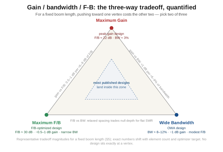
For any fixed boom length, gain, bandwidth, and F/B are genuinely in tension, and the seed chapter’s instinct to draw this as a triangle was the right one — it simply drew it in ASCII art with no numbers attached. The figure below puts real, representative magnitudes on the three vertices and the edges between them:
Three named design philosophies sit near (not at) the three vertices, and each is a real, commercially and academically documented approach rather than a hypothetical extreme:
- Peak-gain optimization pushes every element length and spacing toward the single objective of maximum forward gain at the design frequency. The result typically lands around 22 dB of F/B and a 2:1-SWR bandwidth on the order of 3% of the design frequency — narrow enough that a peak-gain design is usually a single-purpose, single-mode antenna (e.g., tuned for the CW segment of a band and accepting degraded performance elsewhere in it).
- F/B optimization accepts roughly 0.5–1 dB less forward gain than the peak-gain design on the same boom in exchange for pushing the rear null toward 30 dB, and (per §3) typically narrows the usable bandwidth further still, since the rear-null mechanism is itself frequency-sensitive.
- Bandwidth optimization — the OWA (Optimized Wideband Antenna) approach, originated by Jim Breakall (WA3FET) at Penn State using NEC-based global optimization and later adopted by M2 Antennas and others — relaxes element spacing and detunes individual elements slightly off their gain-optimal lengths specifically to flatten the impedance and pattern behavior across a wider slice of spectrum, typically reaching roughly 7% 2:1-SWR bandwidth — Vol 3 §9 traces the commonly-repeated “8–12%” figure to a conflation of two different design traditions at a cost of roughly 1 dB of peak gain and a moderate (rather than maximized) F/B.
Reading the edges of the triangle rather than just the vertices is where the quantitative payoff is: moving from a peak-gain design toward an F/B-optimized one on the same boom costs roughly 0.5–1 dB of gain per 5–8 dB of F/B improvement gained past the 22–25 dB mark, while moving toward an OWA design costs roughly 1 dB of gain per 5–9 percentage points of added 2:1-SWR bandwidth. Most published, buildable designs — the DL6WU tradition, K1FO’s variants, the commercial LFA and OWA product lines — do not sit at any single vertex; they land somewhere in the interior, having made an explicit, named compromise among the three. Reading a manufacturer’s or a published design’s stated gain, F/B, and bandwidth together (rather than any one figure in isolation) tells you which corner of this triangle that particular antenna was built to favor.
2.6 Beamwidth by element count — and the aiming consequence
Half-power beamwidth (HPBW) is the flip side of gain: an antenna concentrates its 2.15 dBi-over-isotropic dipole reference into a progressively narrower solid angle as elements (and boom length) are added, and the narrower that angle gets, the less room there is for aiming error before the signal drops noticeably. Representative HPBW figures by element count (azimuth, horizon-mounted, typical amateur VHF+ designs):
Table 5 — Half-power beamwidth (HPBW) is the flip side of gain: an antenna concentrates its 2.15 dBi-over-isotropic dipole reference into a progressively narrower solid angle as elements (and boom length) are added, and the narrower that angle gets, the less room there is for aiming error before the signal drops noticeably. Representative HPBW figures by element count (azimuth, horizon-mounted, typical amateur VHF+ designs)
| Elements | Azimuth HPBW | Elevation HPBW | Side lobes |
|---|---|---|---|
| 2 | 75° | wide | not meaningful |
| 3 | 60° | ~75° | ~−10 dB |
| 5 | 50° | ~60° | ~−12 dB |
| 7 | 42° | ~52° | ~−14 dB |
| 9 | 35° | ~45° | ~−15 dB |
| 15 | 22° | ~28° | ~−18 dB |
| 28 | 12° | ~16° | ~−20 dB |
The figure below overlays the azimuth pattern shape for four representative element counts (3, 5, 9, and 15) on a common relative-dB polar scale — each normalized to its own peak, so the comparison is of shape (main-lobe width and rough side-lobe/rear behavior), which is what the beamwidth table above quantifies:
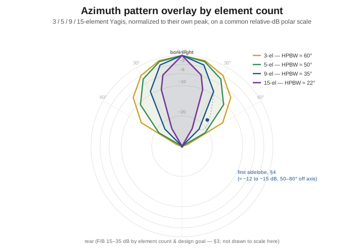
The aiming consequence is direct and worth stating in numbers rather than “narrower is trickier.” A 15-element Yagi’s 22° HPBW means the signal is down 3 dB at just ±11° off boresight; a 30° aiming error — not an unusual amount for a hand-set or poorly-calibrated rotator — puts the actual pointing angle well outside the half-power window entirely. Vol 4 works this rigorously with the standard parabolic pointing-loss approximation L(dB) ≈ 12·(θ/HPBW)², and the answer is worse than a casual estimate suggests: 12·(30/22)² is 22 dB, which is to say the antenna is off its main lobe altogether and what remains is sidelobe response, realistically some 18 dB down. That is not “losing part of the boom’s advantage” — it is losing the antenna. A 5-element Yagi’s 50° HPBW is far more forgiving of the same 30° error, costing about 4.3 dB by the same formula. This is precisely why serious EME and DX operators pair long-boom, narrow-beamwidth Yagis with rotators specified to a couple of degrees of pointing accuracy and a controller with calibration features, while a casual VHF operator working a known repeater or a handful of regular contacts is often better served by a shorter, wider-beamwidth Yagi on a light-duty rotator (or no rotator at all, fixed on the one heading that matters most) than by chasing the last few dB of a long-boom design that then goes chronically mis-aimed. The rotator selection, mounting hardware, and pointing-accuracy discussion that this beamwidth table sets up belongs to Vol 4, which owns installation hardware; this volume’s job ends at establishing the beamwidth-versus-element-count numbers and their aiming cost.
2.7 Stacking as the alternative to a longer boom
Every gain figure in §2 has a mechanical and electrical cost attached to it — more boom, more elements, more wind load, and (per §6) a narrower beamwidth that demands better aiming. Past a certain point, the operator’s actual constraint is rarely “can I model a longer Yagi” and much more often “can I put up a longer boom, and can my tower and rotator carry it.” Stacking — running two (or four) identical Yagis in parallel, fed in phase, separated vertically or horizontally by a carefully chosen distance — is the standard alternative once that mechanical ceiling is reached, and EME and meteor-scatter stations reach for it routinely rather than as a last resort.
2.7.1 The 3 dB from doubling, and what it actually requires
Two identical antennas fed with equal amplitude and the correct phase, combined without loss in the combining network, add 3 dB over a single antenna — twice the radiated power in the favored direction from twice the aperture, the standard two-element array-factor result. In practice the achieved gain is a bit under a clean 3 dB, because a real power-divider network and phasing harness are not perfectly lossless and not perfectly matched, but 2.5–2.8 dB of real, measured improvement from a well-built two-antenna stack is a realistic expectation, and it is a substantial, genuinely useful gain step for the cost of a second antenna and a feed network — not merely “the same gain as adding elements to one boom,” because it comes packaged with a specific, favorable side effect developed in §7.3.
2.7.2 Optimum stacking distance — and why it tracks beamwidth
The stacking distance is not a free parameter to be maximized; there is a real optimum, and it depends directly on the individual antenna’s own beamwidth in the stacking plane. Too close together, and the two antennas’ patterns barely separate — you gain little over a single antenna because the array factor’s own beamwidth is far broader than either antenna’s pattern, and mutual coupling between the two booms can actually degrade the individual antennas’ own patterns. Too far apart, and the array factor develops grating lobes — secondary, nearly-full-strength peaks at other elevation (or azimuth) angles that rob gain from the intended main lobe and radiate a fraction of the power somewhere you did not intend it to go.
A widely-used design rule ties the optimum center-to-center spacing directly to the individual antenna’s half-power beamwidth in the stacking plane: for a typical amateur Yagi with moderate (13–17 dB down) side lobes, S (in λ) ≈ 51 / BW (in degrees); for an unusually clean, low-side-lobe design (side lobes ≥18 dB down), the constant rises to about 57. Those two constants circulate widely in the VHF stacking literature, but this volume could not trace them to a single primary publication — treat them, like the beamwidth and F/B tables above, as a representative design rule rather than an independently sourced result, and prefer a NEC model of your actual pair when the last fraction of a dB matters. Applying that rule to the beamwidth table in §6 (using the elevation HPBW, since vertical stacking is by far the more common arrangement for gain, and it is the elevation-plane pattern that a vertical stack’s array factor multiplies against):
Table 6 — A widely-used design rule ties the optimum center-to-center spacing directly to the individual antenna's half-power beamwidth in the stacking plane: for a typical amateur Yagi with moderate (13–17 dB down) side lobes, S (in λ) ≈ 51 / BW (in degrees); for an unusually clean, low-side-lobe design (side lobes ≥18 dB down), the constant rises to about 57. Those two constants circulate widely in the VHF stacking literature, but this volume could not trace them to a single primary publication — treat them, like the beamwidth and F/B tables above, as a representative design rule rather than an independently sourced result, and prefer a NEC model of your actual pair when the last fraction of a dB matters. Applying that rule to the beamwidth table in §6 (using the elevation HPBW, since vertical stacking is by far the more common arrangement for gain, and it is the elevation-plane pattern that a vertical stack's array factor multiplies against)
| Elements | Elevation HPBW | Optimum stacking distance S ≈ 51/HPBW |
|---|---|---|
| 5 | 60° | ~0.85λ |
| 9 | 45° | ~1.13λ |
| 15 | 28° | ~1.82λ |
| 28 | 16° | ~3.19λ |
The pattern is exactly what the mutual-coupling and grating-lobe reasoning predicts: a wider-beamwidth (shorter-boom) individual antenna needs closer stacking, while a narrower-beamwidth (longer-boom) individual antenna needs to be stacked further apart to avoid the array factor developing grating lobes inside that narrower main beam. This is the direct answer to why stacking distance “depends on the individual antenna’s beamwidth” — it is not an independent mechanical choice, it is set by matching the array factor’s own beamwidth to the pattern it is multiplying against.
2.7.3 The elevation-pattern payoff — why EME and meteor-scatter operators specifically want this
Stacking two Yagis vertically does something a single longer boom cannot: it sharpens the antenna’s pattern specifically in the elevation plane, narrowing the vertical beamwidth beyond what either individual antenna achieves on its own, because the array factor (itself a function of vertical spacing) multiplies against each antenna’s own already-narrow elevation pattern. Working a concrete, illustrative example: a single Yagi with a 45° elevation HPBW (the 9-element figure from §6’s table — note that §6’s 35° for that design is the azimuth number, and vertical stacking multiplies against the elevation pattern), stacked at the S ≈ 1.13λ distance §7.2’s rule gives for that beamwidth, has an array factor of its own with roughly a 25.6° half-power width (solving cos(π·(D/λ)·sinΔ) = 0.707 for D = 1.13λ gives a half-power angle of about 12.8°, or ≈25.6° full width). Combining the single antenna’s own 45° pattern with the array factor’s 25.6° pattern in quadrature — a standard approximation for combining two roughly-independent beamwidth-limiting factors — gives a combined elevation HPBW of about 22°, narrower than either the single antenna’s own pattern or the array factor alone:
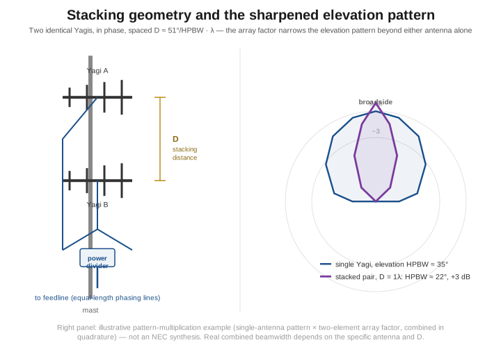
This sharpened elevation pattern is exactly the property EME and meteor-scatter operators are actually buying when they stack, more than the raw 3 dB itself. An EME path looks at a fixed, low elevation angle (the moon’s position at the operating time), and a narrower elevation beamwidth concentrates the antenna’s sensitivity more tightly on that angle, reducing the ground-noise and sky-noise pickup from elevation angles the path does not use — directly complementary to the side-lobe-suppression concern of §4. Meteor-scatter paths similarly benefit from a pattern that discriminates more sharply against unwanted elevation angles while adding gain on the useful ones. A single longer boom on the same frequency would add comparable forward gain, but it sharpens the azimuth pattern (§6) far more than it touches the elevation pattern at a fixed antenna height — the two approaches to “more gain” are not interchangeable in what they do to the pattern shape, and for EME/meteor-scatter work specifically, vertical stacking’s elevation-sharpening is the more directly useful effect of the two.
2.7.4 The honest cost/benefit against a longer boom
Stacking is not free, and the decision against simply building a longer single boom should be made with the real costs on the table. A stacked pair requires twice the antenna hardware — twice the elements, twice the boom, twice the mounting hardware and wind-load calculation — plus a power divider (commonly a simple 1/4-wavelength-transformer or Wilkinson-style splitter, impedance-matched into the combined 50 Ω system) and a phasing harness built to strict, matched electrical length between the two antennas, because any length mismatch introduces a phase error that directly degrades both the array gain and the elevation-pattern sharpening §7.3 describes. Comparing directly: taking a 9-element, 2.2λ-boom Yagi (§2’s table: ~13.35 dBi) and doubling its boom to roughly 4.4λ (a 15–16-element-class design, using the corrected formula from §2.4: 10·log₁₀(4.4) + 9.15 ≈ 15.6 dBi) reaches almost exactly the same gain as stacking two of the original 9-element antennas (13.35 + 3 ≈ 16.35 dBi) — but the longer-single-boom route needs one rotator, one feedline, and no phasing harness, while the stacked route needs two full antennas and the associated combining hardware. The longer boom is very often the cheaper and mechanically simpler route to the same gain number.
The decision genuinely turns on what is actually constrained at the installation site, not on which approach is “better” in the abstract:
- Horizontal space and a rotator/tower rated for a longer boom’s wind load, but no room or desire for a second full antenna: extend the boom.
- Vertical mast space and rotators (or a fixed heading) available for two antennas, and specifically an elevation-pattern benefit wanted (EME, meteor scatter): stack two.
- Needing roughly +6 dB rather than +3: a 2×2 stack (four antennas) is the standard EME-array configuration, combining both vertical and horizontal stacking and requiring proportionally more combining hardware — the mechanical and cost commitment scales accordingly, and this is squarely the territory of dedicated EME and contest installations rather than a casual upgrade.
2.8 Where this volume hands off
This volume corrected the boom-length/gain relationship the seed chapter got wrong — not by inventing a new number, but by checking the claimed formula against its own table (finding a sign-changing error at the short-boom end), checking it against independently NEC-modeled long-Yagi data (finding it holds to within about a dB from roughly 1λ to 8–10λ of boom), and explaining the physical reason the two regimes differ: mutual coupling among a handful of elements below about 1λ, versus the end-fire, traveling-wave aperture behavior above it that Ehrenspeck and Poehler’s 1959 analysis formalized. It also flagged that the seed’s own three internal accounts of this relationship — the per-director list, the “3 dB per doubling” table, and the main gain table — do not agree with each other, by amounts ranging from a few tenths of a dB to a full decibel.
From there, this volume worked outward through the pattern properties that boom length and element count jointly determine: front-to-back ratio and its typical values by element count (§3), the cost of pushing F/B past about 30 dB in gain and bandwidth; side-lobe level and the specific applications — EME, radio astronomy — where suppressing it outweighs peak gain (§4); the three-way gain/bandwidth/F-B tradeoff rendered as a real, quantified triangle rather than ASCII art (§5); half-power beamwidth by element count and its direct, quantified aiming-error cost (§6); and stacking as the mechanical alternative to a longer boom, including the beamwidth-dependent optimum spacing formula, the elevation-pattern sharpening that specifically serves EME and meteor-scatter work, and an honest comparison against simply extending the boom (§7).
What this volume did not cover, by design, belongs to the rest of this dive. Vol 3 takes up the feedpoint-impedance problem Vol 1 quantified and works through the matching-network survey — direct, gamma, hairpin, T-match, and the loop-fed LFA driven element — that turns a Yagi’s collapsed driven-element impedance into a 50 Ω feed, alongside the single-band/OWA/LFA/quagi topology comparison as a building-and-buying decision rather than the pattern-tradeoff physics covered here, and the frequency-response and SWR-bandwidth curve in its own right. Vol 4 takes this volume’s gain, pattern and beamwidth numbers and turns them into an operator’s decision — best- and worst-case use worked through their real mechanisms, the aiming discipline that follows directly from §6’s beamwidth table, rotator selection driven by wind load and turning moment rather than by gain, and power handling from element to feedline. Vol 5 closes the dive with the hands-on side: the DIY build of a 5-element 2 m Yagi, a ranked commercial-buy survey, the companion gear every installation depends on, and the gotchas that catch a first build.
2.9 Resources
- Ehrenspeck, H. W., and Poehler, H., “A New Method for Obtaining Maximum Gain from Yagi Antennas,” IRE Transactions on Antennas and Propagation, October 1959, pp. 379–386 — the original surface-wave/phase-velocity analysis behind the traveling-wave picture of a long Yagi, and the theoretical basis for gain scaling systematically with array length once the array is long enough to behave as an end-fire aperture.
- Cebik, L. B. (W4RNL), “70-CM Yagi Stacks Part 1: 10- to 40-Element DL6WU Examples” — the NEC-modeled DL6WU-tradition gain-vs-boom-length data (12/19/26/32-element, 432 MHz) used in §2.4 to validate the corrected formula’s domain against real, independently-published figures.
- ARRL Antenna Book (25th+ ed.), the Yagi-Uda chapter — the canonical amateur reference for gain-vs-boom-length tables, F/B and side-lobe design tradeoffs, and stacking-distance guidance.
- DL6WU (Günter Hoch) and K1FO (Steve Powlishen) published long-boom Yagi designs — the practical design tradition behind the long-boom NEC data cited in §2.4, and (K1FO specifically) the side-lobe-and-F/B-optimized variant of the DL6WU approach referenced in §5.
- cb-antennas.com, “Gain versus Boom Length” — a hobbyist compilation of over 40 NEC/AN-SOF-modeled Yagi designs, cited in §2.4 for the observation that well-optimized designs at a given boom length typically agree to within about 1 dB of each other; a useful corroborating data point, not a substitute for the peer-reviewed and NEC-modeled sources above.
- Balanis, Antenna Theory: Analysis and Design (4th ed.) and Stutzman & Thiele, Antenna Theory and Design (3rd ed.) — the academic treatment of end-fire array directivity, half-power beamwidth, and the array-factor mathematics behind the stacking-distance and elevation-pattern-sharpening development in §7.
- L. B. Cebik (W4RNL) antenna-modeling papers, more broadly — the deepest amateur-literature treatment of Yagi gain-vs-length, side-lobe behavior, and stacking, archived across the antenna-modeling community.
Comments (0)