Loss, and Where to Put the Tuner

---

3.1 About this volume

This is the volume the dive exists for. Vol 1 showed that a tuner reaches only the impedance at its own input, and closed by demonstrating that every quantity visible from the operating position gets better as the system gets worse. Vol 2 derived the topologies and showed that a T-network matches at many settings that are not equivalent. Both left the same question open: how much does any of this actually cost, and what should you do about it?

The answer has been available in the amateur literature since 1997 and has not displaced the folklore, which is a table of “typical tuner loss” indexed by SWR. Something like this appeared in the previous edition of this chapter:

Table 1 — The answer has been available in the amateur literature since 1997 and has not displaced the folklore, which is a table of "typical tuner loss" indexed by SWR. Something like this appeared in the previous edition of this chapter

mismatch ratio	typical tuner loss (T-network)
2:1 SWR	0.2–0.5 dB
5:1 SWR	0.5–1.0 dB
10:1 SWR	1.0–2.0 dB
20:1 SWR	2.0–4.0 dB
50:1 SWR	4.0–6.0 dB

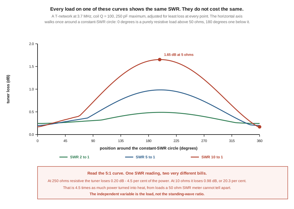
Tables of this shape are everywhere. They are unattributed, they look authoritative, and they are indexed against a variable that does not determine the answer. The same 5:1 SWR can be a 250 Ω load or a 10 Ω load, and the same tuner matching each of them at its best setting loses 0.20 dB in the first case and 0.98 dB in the second — four and a half times the power, from two loads a 50 Ω SWR meter cannot distinguish.

Three results in this volume are worth stating up front.

The first is that the error compounds with severity. §3 walks the load once around each of three constant-SWR circles and finds the spread in loss growing as the mismatch does: a factor of 2.0 at 2:1, 4.5 at 5:1, 8.3 at 10:1. The SWR-indexed table is least reliable exactly where an operator is most likely to consult it.

The second is that the standard feedline formula makes the identical mistake, and this one is the ARRL’s own. §5 shows that the familiar “additional loss due to SWR” calculation is exact for an idealised cable — and that real coaxial cable at HF has a characteristic impedance with a small negative reactive part, which breaks the relationship. On a worked example the formula’s error reaches 0.47 dB and changes sign, and over short runs the true loss is below the matched-line loss, which no formula in SWR alone can produce.

The third is that the shack-versus-mast-base decision is usually framed on the wrong variable too. §6 computes it. The remote tuner’s value is not set by feedline length — it is set by the SWR on the feedline, with length as a multiplier. A 25 ft run at 74:1 justifies a remote tuner more than a 300 ft run at 5:1 does.

One thing this volume is careful not to do is over-correct. The previous edition’s numbers are, for the most part, not fabricated. They are under-specified, which is a different and more interesting failure, and §2 makes the case.

3.2 Three loss tables, three missing variables

Before replacing the previous edition’s figures it is worth working out what was actually wrong with them, because the pattern turns out to be consistent and it names the volume’s subject precisely.

The tuner-loss table omits the load. That is §3 and §4’s subject and the largest of the three.

The feedline table omits the frequency. The previous edition gave coaxial loss over a 30 m run at 1:1 and at 10:1 SWR for four cable types, with no frequency stated anywhere. Coaxial loss goes roughly as the square root of frequency, so a figure without one is not a claim about anything. Computing the LMR-400 row from the manufacturer’s own attenuation formula — 0.122290·√f + 0.000260·f dB per 100 ft, taken from the Times Microwave datasheet rather than a secondary table — gives:

Table 2 — The feedline table omits the frequency. The previous edition gave coaxial loss over a 30 m run at 1:1 and at 10:1 SWR for four cable types, with no frequency stated anywhere. Coaxial loss goes roughly as the square root of frequency, so a figure without one is not a claim about anything. Computing the LMR-400 row from the manufacturer's own attenuation formula — 0.122290·√f + 0.000260·f dB per 100 ft, taken from the Times Microwave datasheet rather than a secondary table — gives

frequency	matched loss over 30 m	at 10:1 SWR
3.5 MHz	0.23 dB	0.86–1.17 dB
7 MHz	0.32 dB	1.29–1.47 dB
14 MHz	0.45 dB	1.79–1.93 dB
28 MHz	0.64 dB	2.44–2.49 dB

The previous edition’s row said 0.3 dB and 1.5 dB. Those are the 7 MHz values. The table is a 40 m table that never says so, and read on 10 metres it understates by a factor of two.

The tuner-versus-coax comparison omits the frequency as well. Its worked example — 20 m of LMR-400, 5:1 SWR, “coax loss ≈ 0.5 dB” — computes to 0.49–0.57 dB at 7 MHz, 0.69–0.77 dB at 14 MHz, and 0.99–1.03 dB at 28 MHz. Again correct on 40 m and nowhere else.

⭐ So the characteristic failure of this chapter’s loss material is not invention. It is quoting a result against an incomplete set of variables — and then, because the number is right in one case, never noticing. That is a subtler and more instructive problem than a wrong figure, and it is worth carrying as a reading habit: when a loss figure is quoted, ask what it is a function of, and whether all of those were stated.

One incidental warning belongs here, since it comes from the same datasheet. LMR-400 and LMR-400-UF are different cables. The ultra-flex version’s attenuation coefficients are 0.146748 and 0.000312 against the standard cable’s 0.122290 and 0.000260 — about 20 % more loss, on a part number that differs by two letters.

3.3 The same SWR, two very different bills

Now the main result. The lead figure holds the standing-wave ratio constant and varies everything else.

A given SWR corresponds not to a load but to a circle of loads — every impedance on that circle produces the same reflection coefficient magnitude and therefore the same meter reading. Walking once around such a circle sweeps from a purely resistive load above 50 Ω, through inductive and capacitive combinations, to a purely resistive load below 50 Ω, and back. The figure computes the T-network’s least-loss setting at every point around three of those circles.

Table 3 — 3. The same SWR, two very different bills

SWR	best case	worst case	power lost, best	power lost, worst
2:1	0.24 dB at 100 Ω	0.49 dB at 25.6 − j6.9	5.5 %	10.7 %
5:1	0.20 dB at 250 Ω	0.98 dB at 10.2 − j7.6	4.5 %	20.3 %
10:1	0.17 dB at 500 Ω	1.65 dB at 5.1 − j7.8	3.8 %	31.7 %

Three things are worth drawing out.

The spread grows with the mismatch. At 2:1 the worst case costs twice the best; at 10:1 it costs more than eight times. A table indexed by SWR is therefore least trustworthy at exactly the mismatches that make someone reach for it — nobody looks up the loss at 2:1.

The low-resistance side is where the cost lives. Every worst case sits near 180° on the circle, which is the purely-resistive-and-below-50-Ω region. Every best case sits at 0°, resistive and above. The asymmetry is complete and it has a mechanism, which §4 gives.

The best cases barely move. As the SWR worsens from 2:1 to 10:1, the best achievable loss actually falls slightly, from 0.24 dB to 0.17 dB. A tuner presented with 500 Ω — nominally a 10:1 mismatch — has an easier job than one presented with 100 Ω at 2:1. Stated as a headline: going from a 2:1 mismatch to a 10:1 mismatch can reduce your tuner loss, if the direction is right. That sentence is nonsense in the SWR-indexed picture and obvious in the correct one.

3.4 Loss against the load, which is the table that works

Replacing the wrong table means plotting against the right variable.

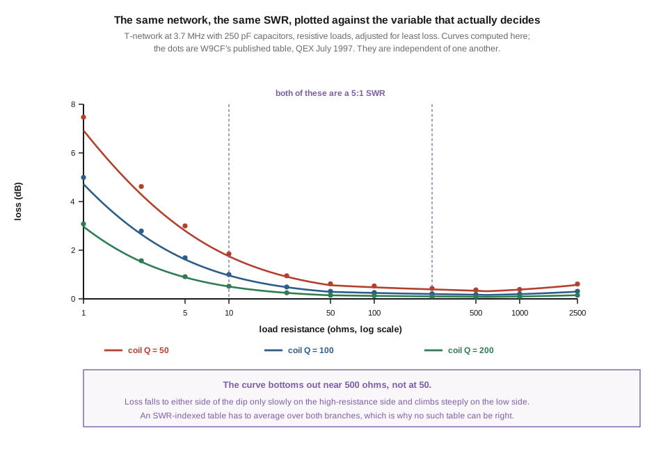
The curves are computed from the network equations; the dots are Kevin Schmidt W9CF’s published table, from Estimating T-network losses at 80 and 160 meters (QEX, July 1997). They were arrived at independently and they agree, which is worth more than either alone. The key rows, quoted from his table:

Table 4 — The curves are computed from the network equations; the dots are Kevin Schmidt W9CF's published table, from Estimating T-network losses at 80 and 160 meters (QEX, July 1997). They were arrived at independently and they agree, which is worth more than either alone. The key rows, quoted from his table

load R	SWR	Q = 50	Q = 100	Q = 200
1 Ω	50:1	7.47 dB	4.99 dB	3.08 dB
5 Ω	10:1	3.00 dB	1.69 dB	0.91 dB
10 Ω	5:1	1.85 dB	1.00 dB	0.52 dB
50 Ω	1:1	0.62 dB	0.31 dB	0.15 dB
250 Ω	5:1	0.43 dB	0.21 dB	0.10 dB
500 Ω	10:1	0.37 dB	0.18 dB	0.08 dB
2500 Ω	50:1	0.61 dB	0.31 dB	0.15 dB

Read the SWR column and the loss columns together and the point is unmissable. Every SWR value in that table appears twice, with losses differing by a factor of four to sixteen.

3.4.1 The mechanism, and where the coil’s resistance actually bites

Vol 2 §4 established the structural fact, in W9CF’s words: “any T-network will transform the load resistance to a higher value which must also be higher than 50 ohms. It then transforms this high value down to 50 ohms to produce a match.” The loss follows directly, and it is worth spelling out as a chain because the seed’s account — “the Q × resistance product dissipates more power per dB of forced match” — named no mechanism at all.

A real inductor is an inductance in series with a small resistance, its equivalent series resistance. Referred to the node it sits across, that appears as a large parallel resistance of roughly Q·X_L, which for a good roller inductor at HF is ten to twenty thousand ohms. The fraction of power lost in the network is essentially the ratio of the node’s impedance to that parallel resistance. So:

• A low-resistance load forces a high intermediate impedance. W9CF’s worked case is a 10 Ω load at 80 m transformed to a 4 000 Ω parallel equivalent. Against a coil parallel resistance of 10–20 kΩ, that is “of order 10 percent” of the power gone.
• A high-resistance load does not. Matching 500 Ω requires much less transformation, the node sits lower, and the coil’s loss resistance is a smaller fraction of it.

Equivalently, in current terms: the operating Q of the network is the ratio of circulating current to load current, and the loss is I²R in the coil’s series resistance. Forcing a large impedance transformation raises the circulating current, and the heating goes as its square. That is the whole of the “operating Q” story, and it is the same physical quantity that produced Vol 2’s 6 800 V at the shunt node — high circulating current in a high reactance is simultaneously a heating problem and a voltage problem.

⭐ One consequence is counter-intuitive enough to state on its own: the loss curve bottoms out near 500 Ω, not at 50 Ω. A T-network matching 500 Ω to 50 Ω loses less than the same network matching 50 Ω to 50 Ω. The reason is that a T-network cannot do nothing — presented with a matched load it still transforms up and back down, and at 50 Ω that round trip is more work than the one 500 Ω asks for. It is a small effect, 0.31 dB against 0.18 dB, but it is a clean demonstration that the network’s cost is a function of where the load is, not of how far the load is from ideal.

3.4.2 The L-network comparison, which the previous edition got right

The previous edition also printed a second table asserting that an L-network loses less than a T-network for the same match. That claim is correct, it has a clean mechanism, and it deserves to survive the demolition of the table it appeared in.

W9CF derives it and states the consequences compactly: the L-network is better “by an overall factor of |X_C2|/R_0 which is about a factor of 7 for C_max of 250 pF at 160 meters. In addition, the loss for a load of 50 ohms is zero (where the L and C values are both zero) and it increases slower with SWR than for the T networks. The penalty is the limited matching range.”

Computing both networks at 3.7 MHz with a coil of Q = 100:

Table 5 — Computing both networks at 3.7 MHz with a coil of Q = 100

load R	SWR	L-network	T-network
5 Ω	10:1	0.128 dB	1.621 dB
10 Ω	5:1	0.086 dB	0.964 dB
50 Ω	1:1	0.000 dB	0.289 dB
250 Ω	5:1	0.086 dB	0.200 dB
1000 Ω	20:1	0.185 dB	0.195 dB

Three of W9CF’s four statements are confirmed exactly. The L-network’s loss really does go to zero at a matched load — because at 50 Ω both its elements go to zero and there is no network left, which the T-network can never do. Its loss rises far more slowly with mismatch. And the penalty really is matching range: Vol 2 §6 computed an L-network’s practical span as 52 Ω to 9.6 kΩ against the T’s fraction-of-an-ohm to 19 kΩ, limited by capacitor values rather than by topology.

⚠ The fourth does not reproduce cleanly and is flagged rather than smoothed over. His factor of about 7 at 160 m is |X_C2|/R₀ from his simplified algebra; computing both networks exactly at 1.85 MHz gives a ratio of roughly 20 at low load resistances. The direction and the mechanism agree; the magnitude does not, and the difference is most likely in which T-network setting his approximation compares against. Use his qualitative conclusions, which are solid, rather than the factor of 7.

⭐ One nuance neither source states: the L-network’s advantage is concentrated exactly where the T-network is worst. At 10 Ω it is better by more than eleven times; at 1000 Ω the two are within five per cent of each other. If your loads are high-resistance — an end-fed wire, a doublet on a band where the feeder presents kilohms — the topology choice barely matters. If they are low-resistance, it matters enormously.

3.4.3 What this means at the operating position

Three practical rules fall out, and none of them can be derived from an SWR reading.

A tuner working hard is a tuner running hot at low impedances. If your tuner gets warm, the load is resistive and small — a short antenna, a wire near a half-wave multiple, or a feedline length that has transformed a high impedance to a low one. The fix is usually to change the feedline length, which moves the load around the circle in the lead figure, not to buy a better tuner.

Coil Q is worth more than anything else you can change. Look at the columns: going from Q = 50 to Q = 200 divides the loss by roughly two and a half at every load. That is a bigger effect than any adjustment the operator can make, and it is decided when the tuner is built. W9CF reports W8JI’s estimate for real hardware — “a rough estimate of the Q of high quality, off the shelf, commercial roller inductors would range from a low of around 20 at low values of inductance, up to a maximum Q around 100.” A Q of 20 at the low-inductance end of a roller’s travel is a sobering number, and it is one reason the largest-capacitance rule from Vol 2 matters: it keeps you out of that part of the coil.

The variable you can actually see is the wrong one. This is where the volume rejoins Vol 1 §7. The SWR at the tuner input tells you nothing about which branch of the curve you are on, and the tuner’s own controls do not report the intermediate impedance. Measuring the load — which is Vol 4’s subject — is the only way to know.

3.5 The feedline makes exactly the same mistake

The tuner is not the only place in the system where a loss is routinely computed from an SWR number. The other is the feedline, and there the mistake is enshrined in a formula that has been in the ARRL Handbook for decades.

The “additional loss due to SWR” calculation takes the cable’s matched-line loss and the load’s reflection coefficient magnitude and returns a total loss. Written with a as the matched loss expressed as a power ratio and Γ as the reflection coefficient magnitude:

Total loss (dB) = −10·log₁₀[ a(1 − Γ²) / (a² − Γ²) ]

The first thing to say about it is that for an idealised cable it is not an approximation at all — it is exact. Modelling a line with a purely real characteristic impedance and sweeping the load once around a constant-SWR circle, the total loss is identical at every point: 2.1235 dB at every load phase for a 5:1 SWR on a line of 1 dB matched loss, and the formula returns 2.1235 dB. With a real Z₀, the SWR and the matched loss genuinely do determine the answer.

That is worth stating clearly because it explains why the formula survives, and it also isolates what actually goes wrong.

Real cables do not have a real Z₀. A transmission line’s characteristic impedance is √((R + jωL)/(G + jωC)), and at frequencies where conductor loss dominates it carries a small negative reactive part — approximately Z₀ = R₀(1 − j·α/β), where α is the attenuation constant and β the phase constant. Steve Stearns K6OIK is credited with identifying this as the flaw in the ARRL formula; as Dan Maguire AC6LA puts it, “the characteristic impedance Zo of real transmissions lines at frequencies below the GHz range always has a -jXo component.” For RG-8X at 3.5 MHz the model used here gives Z₀ = 50.0 − j2.32, a reactive part of about 4.6 %.

That is small, and its consequences are not.

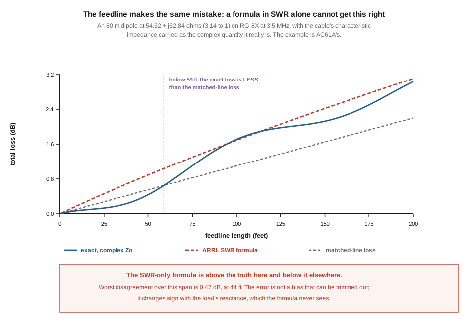
The example is AC6LA’s: an 80 m dipole presenting 54.52 + j62.84 Ω — a 3.14:1 SWR — fed with RG-8X. Computing it exactly against the formula:

• The worst disagreement over a 200 ft span is 0.47 dB, at 44 ft.
• The error changes sign. The formula runs above the truth over most of the range and below it around 100 ft, so it is not a bias that can be corrected with a fudge factor.
• Below 59 ft the true total loss is less than the matched-line loss. AC6LA reports the same effect setting in below 55 feet on the same example — an independent agreement worth noting, since the crossover is the sharpest test of the model.

That last item deserves a moment. A line carrying a 3:1 standing wave, over short runs, loses less than the same line would if perfectly matched. No formula whose only inputs are matched loss and SWR can produce that result, because both of those inputs are monotonic in the direction of more loss. The effect comes entirely from the reactive part of Z₀ interacting with the load’s reactance, and it disappears if you assume that part away.

⭐ The structural point is the volume’s spine appearing a second time. The tuner’s loss was tabulated against SWR and turned out to depend on the load. The feedline’s loss is calculated from SWR and turns out to depend on the load’s reactance and the line’s length. Both are the same error — computing a quantity from a number that summarises away the information the answer needs — and in the feedline’s case the error is published by the organisation whose handbook the hobby treats as canonical.

The practical remedy is not arithmetic. It is to use one of the modelling tools that carries the complex Z₀ properly. AC6LA lists TLDetails, N6BV’s TLW (which ships with the ARRL Antenna Book), EZNEC and AutoEZ; any of them will do, and none of them is harder to use than the formula.

3.6 Where to put the tuner, with numbers

Everything above converges on the one decision an operator actually makes: tuner in the shack, or tuner at the antenna?

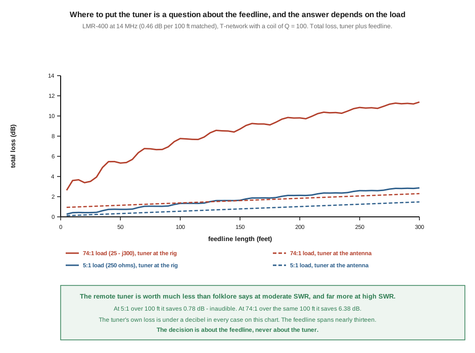
The figure computes both placements. With the tuner at the rig, the feedline runs at the antenna’s SWR and the tuner matches whatever arrives at the shack end. With the tuner at the feedpoint, the tuner matches the antenna directly and the feedline runs at 1:1. Both totals include the tuner’s own loss.

Table 6 — 6. Where to put the tuner, with numbers

load	25 ft	50 ft	100 ft	200 ft	300 ft
250 Ω (5:1)	0.21 dB	0.42 dB	0.78 dB	1.11 dB	1.39 dB
25 − j300 (74:1)	2.48 dB	4.18 dB	6.38 dB	7.97 dB	9.08 dB

Those are the savings from moving the tuner to the antenna.

The previous edition’s rule was framed on length, and said that runs under 15 m are fine at the rig with a penalty under 0.5 dB, while runs over 30 m want a remote tuner. Checked against the top row, that is very nearly right: at 5:1 over 50 ft the saving is 0.42 dB. ⚠ It would be an over-correction to call the rule wrong.

But it is right about the wrong case. The bottom row is a real antenna — a wire that is nowhere near resonant on the band in use, which is precisely the situation that makes someone buy a tuner in the first place. There, a 25 ft run already justifies the remote tuner by 2.5 dB, and the seed’s rule would have told the reader not to bother.

⭐ So the correct rule is not about length. It is about the SWR the feedline is being asked to carry, with length as a multiplier:

• Resonant antenna, tuner trimming band edges (2:1 to 5:1). Keep the tuner in the shack. Even 300 ft of good coax only costs you 1.4 dB, and a remote tuner brings its own failure modes — a relay box up a mast, DC and control over the coax, and weatherproofing.
• Non-resonant wire, doublet on the wrong band, anything above about 10:1. The remote tuner earns its money immediately, at any length worth running.
• Anything in between. Compute it. The two variables are the load and the cable’s loss at the frequency you care about, and §5’s tools do it in a minute.

3.6.1 The third option, which is usually the best one

There is an alternative the framing above hides, and Vol 1’s worked example already contained it.

The reason high SWR is expensive is that it multiplies the feedline’s matched loss. If the matched loss is nearly zero, the multiplication does not matter. G3TXQ’s doublet in Vol 1 §3 ran at 34.2:1 on its 300 Ω ladderline and lost almost nothing, because open-wire line has a matched loss an order of magnitude below coaxial cable at HF.

That is the classic doublet-and-balanced-tuner station, and on these numbers it is not nostalgia. Feeding a non-resonant wire with open-wire line and tuning in the shack can beat both coaxial options, because it attacks the term that all the loss is proportional to rather than trying to get out of its way. The costs are real — the line has to be kept clear of metal, it does not like being coiled or run through walls, and it demands a balanced tuner or a good balun — and they belong to Vol 5, where the hardware is. But the physics is on its side, and any comparison that offers only “tuner at the rig” and “tuner at the mast” has left out the option that wins.

3.7 Where this volume hands off

The chapter’s loss material was not fabricated; it was under-specified, three times in the same way. The tuner table omitted the load, and the load is what decides: at 5:1 the same network loses 0.20 dB into 250 Ω and 0.98 dB into 10 Ω, and the spread grows to more than eight to one by 10:1. The feedline tables omitted the frequency, and were correct on 40 m and nowhere else. The mechanism behind the tuner numbers is ordinary — a T-network transforms the load up before bringing it down, and the coil’s loss resistance sits across whatever node that creates — and it explains the heating and the flashover voltage at once. The standard feedline formula makes the same error the tuner table does, is exact only for a cable with a real characteristic impedance, and misses by up to half a decibel in both directions on a real one. And the placement decision follows the SWR on the line rather than its length, with the open-wire option beating both coaxial answers on the physics.

From here:

• Vol 4 — Finding the load, and matching by hand answers the question this volume raises and cannot settle: if the load is the variable that decides, how do you find out what it is? A VNA sweep at the tuner’s terminals puts you on the correct branch of §4’s curve in about a minute, and the Smith chart turns Vol 2’s algebra into two arcs you can read by eye.
• Vol 5 — DIY build and buys is where §4’s coil-Q finding becomes a purchasing decision, where the balanced-tuner option in §6 gets its hardware, and where the commercial survey lives.
• Vol 1 is worth rereading after this one. Its closing result — that the tuner’s efficiency rises as the system collapses — is the same physics as §3’s, seen from the shack instead of from the bench.

One thing is owed against this volume. Every loss figure here is calculated rather than measured. W9CF’s table is itself calculated, though it agrees with the measurement techniques Frank Witt AI1H and Andrew Griffith W4ULD published in QST and QEX, and an independent bench measurement on a real tuner — the S21 method the NanoVNA dive describes — would be the right way to close the loop. It is a bench task, not a literature one.

3.8 Resources

• Kevin Schmidt, W9CF, Estimating T-network losses at 80 and 160 meters, QEX, July 1997 — the source this volume is built on. The loss-against-load table, the parallel-equivalent mechanism, the largest-capacitance operating rule, and the observation that constant-loss contours on a Smith chart are not the constant-SWR circles. The host it was published on no longer resolves; it survives in the Internet Archive.
• Dan Maguire, AC6LA, “Additional Loss Due to SWR” — §5’s subject: what the ARRL formula is, the worked 80 m dipole example, and the comparison against methods that carry a complex Z₀. Also the source for the tool list.
• Steve Stearns, K6OIK, Facts About SWR, Reflected Power, and Power Transfer (Pacificon 2014, and a later QEX article) — credited by AC6LA with identifying the flawed assumption behind the ARRL formula.
• Charles Michaels, W7XC, QST, November 1997 — the transmission-line-equation method for total line loss that AC6LA validates against.
• Frank Witt, AI1H — QST, April and May 1995, and “Evaluation of Antenna Tuners and Baluns — an Update”, QEX, September/October 2003. How to measure tuner loss rather than calculate it, which is the missing half of this volume.
• Times Microwave Systems, LMR-400 datasheet — the attenuation-versus-frequency coefficients used in §2 and §6, read from the datasheet itself. Note that LMR-400-UF is a different cable with about 20 % more loss.
• Tom Rauch, W8JI, Antenna tuners — realistic roller-inductor Q, and the reminder that near 50 Ω the differences between topologies are small.
• Antenna tuners, Vol 1 — the system-level version of §3’s result, and the doublet whose 34:1 feeder costs almost nothing.
• Random wire and end-fed antennas, Vol 4 — the same tune-at-the-rig versus tune-at-the-antenna argument from the antenna’s side, and the transformer-scale version of loss flatters SWR.
• NanoVNA, Vol 4 — the S-parameter technique for measuring a matching network’s loss on the bench, which is what this volume owes.