DIY Build and Buys

---

5.1 About this volume

Four volumes of theory arrive here. Vol 1 established that a tuner reaches only its own input. Vol 2 derived the topologies and found the previous edition’s two schematics wired backwards. Vol 3 showed that the load, not the SWR, decides the cost. Vol 4 found the same backwards wiring in the Smith-chart procedure and showed how to measure the load that settles it. This volume builds something and buys something.

Both halves needed more correcting than expected, and in opposite directions.

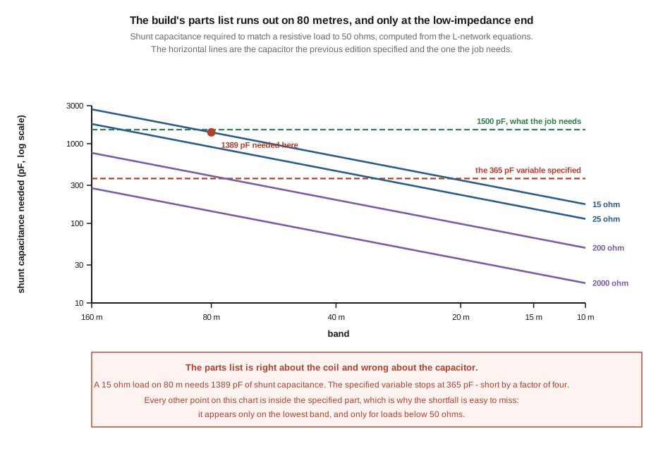
The build’s parts list is mostly right. The 30 µH coil specification — 28 turns of #14 on a 2″ form — computes to 30.7 µH by Wheeler’s formula, which is as close as anyone needs. That is worth saying first, because this dive has spent four volumes correcting things and the temptation to keep finding errors is a failure mode in its own right. One part is wrong, and §2 shows exactly where: the 365 pF shunt capacitor is short by a factor of four, in one corner of the range, on one band.

The schematic is wrong in the way the rest of the chapter is wrong. It draws the shunt element at the antenna and captions it “the shunt-C variable handles low-Z loads” — backwards, for the third time in this chapter, and this time it leaves the finished tuner unable to match anything below 50 Ω on any band. §2 fixes it with a switch.

The test procedure tests nothing. The build is to be verified “with a 50 Ω dummy load on the antenna side” — and a 50 Ω load is the single case that requires no tuner at all. The correct settings are both elements at zero. §4 replaces it.

And the commercial survey describes a market that has partly ceased to exist. MFJ Enterprises stopped manufacturing on 17 May 2024; the previous edition lists eleven MFJ models as current products with 2026 prices. Of the five prices that could be checked against a manufacturer’s own store, five were wrong, by up to 38 %, in both directions. §5 gives what could be verified on 1 August 2026 and hedges the rest explicitly rather than filling the gaps.

5.2 The build, and the one part that is wrong

The target is the previous edition’s: an L-network for 80 through 10 metres at 200 W. Taking the design equations from Vol 2 and asking what components a range of 15 Ω to 2000 Ω actually demands:

Table 1 — The target is the previous edition's: an L-network for 80 through 10 metres at 200 W. Taking the design equations from [Vol 2](/antenna-tuners/vol-2/) and asking what components a range of 15 Ω to 2000 Ω actually demands

band	15 Ω load	200 Ω load	2000 Ω load
80 m	1.04 µH, 1389 pF	3.94 µH, 394 pF	14.20 µH, 142 pF
40 m	0.52 µH, 695 pF	1.97 µH, 197 pF	7.10 µH, 71 pF
20 m	0.26 µH, 347 pF	0.99 µH, 98 pF	3.55 µH, 35 pF
10 m	0.13 µH, 174 pF	0.49 µH, 49 pF	1.78 µH, 18 pF

The worst case across that whole range is 14.2 µH of series inductance and 1389 pF of shunt capacitance, and the two extremes are at opposite corners: the inductance is worst for a high-resistance load on the lowest band, the capacitance for a low-resistance load on the same band.

Against that, the previous edition’s parts:

• Roller or tapped inductor, 30 µH. Correct, with better than 2:1 headroom over the worst case. Wheeler’s formula for 28 close-wound turns of #14 on a 2″ form gives 30.7 µH, so the winding specification is right too.
• Variable capacitors of 200 pF and 365 pF. The 365 pF part is short by a factor of four for a 15 Ω load on 80 m.

The lead figure shows why this is easy to miss. Every other point in the table is comfortably inside 365 pF. The shortfall exists only on the lowest band, only below 50 Ω, and only there — so a builder who tests on 20 m, or with a high-impedance wire, will never meet it.

The fix is a switchable padder, not a bigger variable. Air variables above 500 pF with useful plate spacing are large, expensive and hard to find; two or three fixed capacitors — silver mica or transmitting doorknob types, 1000 V or better — switched in parallel with the variable give you 1400 pF when you need it and get out of the way when you do not. If you want 160 m as well, the worst case rises to 27.6 µH and 2701 pF, which is why the build is specified 80–10 m.

5.2.1 The schematic, and the switch it needs

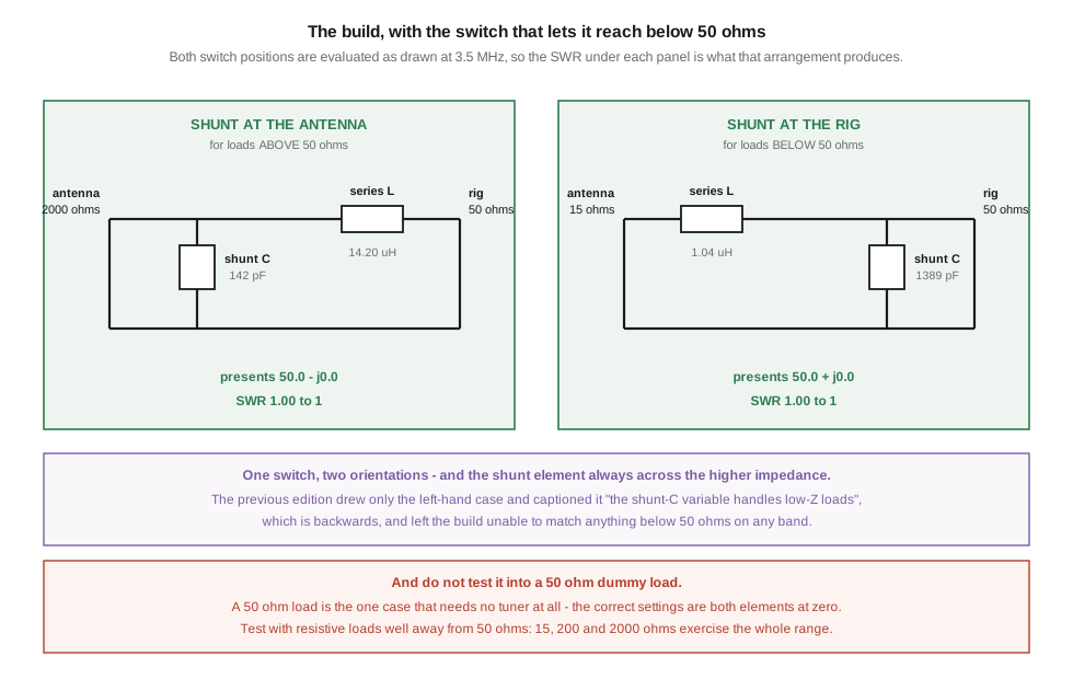
The previous edition drew one circuit: antenna, shunt capacitor to ground, series inductor, series capacitor, rig. The shunt sits at the antenna. Vol 2 established the rule — the shunt element goes across the higher of the two impedances, because it is the only element that transforms resistance and it can only reduce it. So shunt-at-the-antenna is correct for loads above 50 Ω and wrong for loads below.

Evaluating the drawn circuit across its range at 3.5 MHz with the specified parts, it matches 49 Ω to about 8700 Ω — and nothing at all below 50 Ω, on any band. That is half the problem missing from a general-purpose tuner, and it is precisely the half that a short antenna or a wire near a half-wave multiple presents.

Worse, the caption under that schematic reads “The shunt-C variable handles low-Z loads.” It is the opposite: a shunt at the antenna handles high-Z loads. That is the third independent appearance of this inversion in the chapter, after the two schematics in §3 and the Smith-chart procedure in §6.

The fix is one switch. A two-pole changeover that moves the shunt capacitor from the antenna side to the rig side converts a high-Z-only network into one that covers both. The figure draws both positions, and each was evaluated as drawn — 50.0 Ω, 1.00:1, both ways.

5.2.2 Voltage, and what plate spacing you actually need

The previous edition specifies 2 kV air variables and “~2 mm minimum” plate spacing. Checking it: across the 15 Ω to 2000 Ω range at 200 W, the peak voltage across the shunt element reaches about 894 V. A 2 kV part therefore has better than 2:1 margin, and a 2 mm gap — which stands roughly 3 kV under the conservative derating amateurs use for dusty, humid air rather than the 3 kV/mm of dry laboratory air — is comfortable.

⚠ The margin is thin only at the extreme. If you push the network to the top of its 8700 Ω reach, the shunt voltage rises to about 1868 V peak at 200 W, which is nearly all of a 2 kV rating. The honest statement is that the specified parts are right for the specified range and marginal beyond it, and that a flashover is the failure mode you get rather than a warm component.

5.2.3 The bill of materials

⚠ Prices below are estimates, not quotations. The previous edition’s BOM listed a roller inductor at $15, which is not a price any roller inductor has sold for in decades — surplus units run from about $60, and new ones considerably more — and its line items summed to $140 under a heading that said $120. Rather than repeat that with different numbers, this list marks what varies.

Table 2 — The bill of materials

part	specification	note
Variable capacitor	365 pF air variable, 2 kV plate spacing	surplus; the price varies by an order of magnitude
Fixed padders	2 or 3 units totalling ~1100 pF, 1 kV+, silver mica or doorknob	the correction in this section
Variable capacitor	200 pF air variable, 2 kV	for the series position if you build the three-element variant
Inductor	30 µH — 28 turns of #14 enamelled on a 2″ form, tapped, or a roller	the coil spec that was already right
Tap switch	ceramic, 10–12 position, RF-rated	not a general-purpose rotary
Orientation switch	2-pole changeover, ceramic, RF-rated	the part the previous edition omits
Chassis	steel or aluminium, 10″ × 8″ × 4″
Connectors, knobs, hardware	SO-239 in and out, insulated couplers

Budget a few hundred dollars if you buy the variables new and rather less from a hamfest — which is, realistically, where the parts for a project like this come from.

5.3 Construction

Wind the coil first, because its diameter sets the chassis. Twenty-eight turns of #14 enamelled wire close-wound on a 2″ form gives 30.7 µH and occupies about 1.8″. Space-winding raises the Q and lowers the inductance; if you space the turns, re-measure rather than trusting the table. Bring taps out at turns 4, 7, 10, 14, 18, 22 and 28 — the geometric-ish spacing matters more than the exact numbers, because you want roughly equal ratios between adjacent taps rather than equal increments.

Mount the variables on ceramic or PTFE standoffs, not directly to the chassis, and drive them through insulated couplers. The rotor of a capacitor in the shunt position sits at RF ground and the one in a series position does not; an insulated coupler is what stops the front panel from being live.

Keep the leads short and the ground return solid. At 30 MHz an inch of wire is around 20 nΩ… which is to say a few tens of nanohenries, and a few tens of nanohenries is a couple of ohms of reactance. That is small against a 300 Ω node and not small against a 15 Ω one. The low-impedance side of the network is where layout matters.

Fit a common-mode choke at the output. A tuner sits at a point of high voltage and its chassis is a large conductor; without a choke the coax braid becomes part of the antenna and the impedance you measured in Vol 4 §2 will move when you touch things. The BALUNs and UNUNs dive covers the winding; a string of mix-31 beads or a few turns on an FT240-31 at the antenna terminal is the usual answer.

Label the tap positions and the switch, and leave room for a log. §4 explains why.

5.4 Testing it, which the previous edition did not

The previous edition’s verification step is:

Test with a 50 Ω dummy load on the antenna side. Sweep with NanoVNA across 1.8-30 MHz. Adjust the L tap and the two caps for SWR < 1.5:1 at each band.

🔴 A 50 Ω load is the one case that needs no tuner at all. Connect a good dummy load to the antenna terminal and the correct setting is both elements at zero — no inductance, no capacitance, straight through. The test will pass on a tuner whose switch is miswired, whose taps are shorted, or whose capacitors are open, because it never asks the network to transform anything. It exercises exactly the case the device is not for.

This is the same class of error as the bench test the BALUNs and UNUNs dive had to replace, where an SWR check with a dummy load exercised only the differential path and could not see the choking impedance at all. A test that the device passes when broken is worse than no test, because it produces confidence.

5.4.1 What to test instead

Build three resistive test loads: about 15 Ω, 200 Ω and 2000 Ω. Non-inductive resistors — carbon composition or thick-film, never wirewound — in series-parallel to get the values, mounted on a connector with the shortest possible leads. They need to dissipate only the milliwatts a VNA supplies, so quarter-watt parts are fine; this is a measurement fixture, not a dummy load. Those three values bracket the design range and put one point on each side of 50 Ω.

Then, for each load and each band:

1. Verify the load itself with the VNA before you trust anything downstream. A “2000 Ω” resistor assembly has stray capacitance and will not read 2000 + j0 at 28 MHz. Measure it and record what it actually is.
2. Set the orientation switch correctly — shunt at the antenna for the 200 Ω and 2000 Ω loads, shunt at the rig for the 15 Ω one. If the tuner will not match with the switch the “wrong” way, that is confirmation the switch is doing its job.
3. Adjust for a match and record the tap number and both capacitor settings.
4. Measure the insertion loss, which is the number Vol 3 wanted and could not supply. The method is the two-port one from the NanoVNA dive: the network in series between the two VNA ports, complex S21, calibrated through with the fixture shorted. Expect the 15 Ω load to cost several times what the 2000 Ω load costs — that is Vol 3’s whole argument, and your tuner is a chance to confirm it on a bench rather than in a spreadsheet.

⚠ Two claims from the previous edition to discard. “L tap settings: typically tap 5 for 80 m, tap 3 for 40 m, tap 1 for 20-10 m” is invented specificity — the tap depends on the load, not on the band, and this dive’s whole argument is that those are different variables. And “total insertion loss: 0.5-1.0 dB” is a single figure for a quantity that Vol 3 showed varies by a factor of eight with the load at fixed SWR. Measure yours; do not adopt a number.

Keep the log. A table of tap and capacitor settings against band and antenna is what makes a manual tuner fast to use, and it is the thing an autotuner’s memory does for you. It is also how you notice that something has changed.

5.5 The market, dated

Everything in this section was read on 1 August 2026 from the source named. Where a figure could not be verified it is marked as unverified rather than filled in, because the previous edition’s product tables are a demonstration of what happens otherwise.

5.5.1 The largest name in the tables no longer manufactures

MFJ Enterprises ceased on-site production at Starkville, Mississippi on 17 May 2024, announced on 26 April that year, taking Ameritron, Hy-Gain, Cushcraft, Mirage and Vectronics with it. Remaining inventory has continued to sell. On 15 April 2026, ITU Corporation of Linton, Indiana announced it was acquiring the Cushcraft and Hy-Gain brands.

The previous edition lists eleven MFJ tuners — the 902, 925, 929, 948, 962D, 974HB, 976, 986, 989D, 993B and 994B — as current products with mid-2026 prices. Every one of those rows needs reading as a used-market or remaining-stock entry. MFJ tuners are not bad and there are a great many of them in circulation; the correction is that “buy a new MFJ-993B” stopped being advice in May 2024.

5.5.2 Verified prices

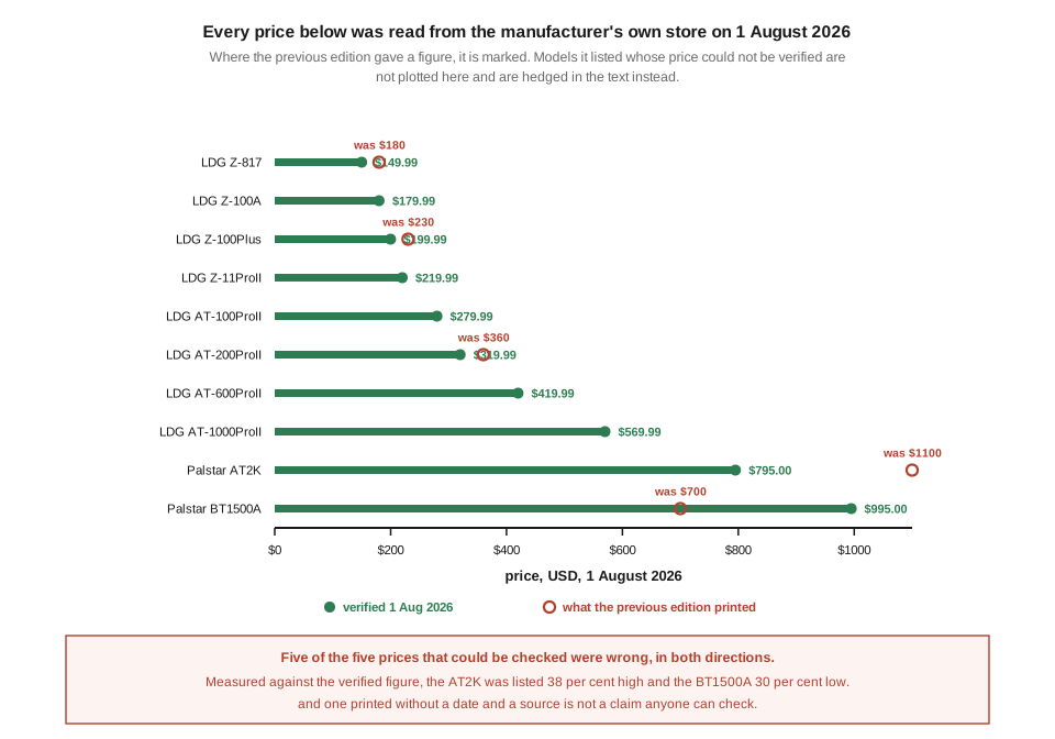
Table 3 — Verified prices

model	price, 1 Aug 2026	source	previously printed
LDG Z-817	$149.99	LDG	$180
LDG Z-100A	$179.99	LDG	not listed
LDG Z-100Plus	$199.99	LDG	$230
LDG Z-11ProII	$219.99	LDG	not listed
LDG AT-100ProII	$279.99	LDG	no price
LDG AT-200ProII	$319.99	LDG	$360
LDG AT-600ProII	$419.99	LDG	no price
LDG AT-1000ProII	$569.99	LDG	not listed
Palstar AT2K	$795.00	Palstar	$1100
Palstar BT1500A	$995.00	Palstar	$700

Five of the five prices that could be checked were wrong, and not in a consistent direction: measured against the verified figure, the AT2K was listed 38 % high and the BT1500A 30 % low. ⭐ A price list without a date and a source is not a claim anyone can check, which is the reason this one carries both.

5.5.3 What changed, model by model

LDG is active and its Maryland operation continues. Two corrections to the previous edition’s account. Its flagship recommendation, the Z-100Plus, is still sold at $199.99 — so listing it was not wrong — but LDG now also sells the Z-100A at $179.99 alongside it, and the previous edition does not mention it. And the current remote model is the RT/RC-100; the “RT-200” the previous edition lists does not appear in LDG’s line.

Palstar AT2K is current at $795.00 and covers 160 through 6 metres — the previous edition’s “1.8–30 MHz” omits 6 m. Palstar offers an optional external 4:1 or 1:1 current balun for balanced feeders rather than building one in.

Palstar BT1500A is current at $995.00, and its specification carries a detail the previous edition flattens away: its matching range is band-dependent. Palstar states 2500 ± j2500 Ω on 20 through 160 m, and 1000 ± j1000 Ω on 10 and 15 m. A single “1.8–30 MHz” row hides that the high bands get less than half the reach.

⭐ And the BT1500A confirms a claim from the previous edition’s myth list that was worth confirming. It says of balanced tuners that “balanced tuners use BALUNs internally — typically false. Modern balanced tuners use differential L-networks.” Palstar describes the BT1500A as “the only 1500 Watt, Double-L Network antenna tuner on the market today” with “two tandem mounted, precision ceramic roller inductors for a truly balanced tuner”, explicitly not a balun design. The myth-busting entry stands.

Icom AH-4 covers 3.5–54 MHz with a wire of at least 23 ft, choosing from over 1,040,000 LC combinations and memorising 45 frequencies — the previous edition’s band figures for it are correct.

Icom AH-705, the IC-705’s companion, covers 160 m through 6 m. The previous edition gives “0.5–30 MHz” in two places, which is wrong at both ends.

Yaesu FC-40 covers 1.8–54 MHz with a wire longer than 66 ft, or 7–54 MHz with an 8 ft whip, and holds 200 match memories. The previous edition’s “1.8–30 MHz” understates it.

Elecraft continues to sell both the KAT500 and the T1, the latter in assembled and kit forms. ⚠ Neither price could be read from Elecraft’s own pages, and neither is quoted here. The previous edition gives $700 and $200; those figures are unverified and should be treated as such until someone checks them.

SGC’s SG-237 and SG-239 show as no longer available at European retailers. ⚠ SGC’s own position was not established, so this is a distribution observation rather than a discontinuation notice.

5.5.4 What to avoid, which the previous edition got right

Its three warnings all survive scrutiny, and this dive has now supplied the mechanisms behind them:

• “Very small autotuners claiming kW ratings — variable-capacitor voltage breakdown is the failure mode; physical size dictates voltage handling.” Correct, and Vol 2 put a number on it: a T-network matching a 10 Ω load at 3.7 MHz stands 6800 V RMS at its shunt node for 100 W. Voltage, not heat, is what kills small tuners.
• “Autotuners without published SWR/loss specs.” Correct, and Vol 3 explains why a published figure is worth so much: loss is a function of the load, so a manufacturer willing to state it has had to say at what load.
• “‘Universal autotuners’ matching 1 Ω to 10 kΩ — physically impossible without significant loss at the extreme ratios.” Correct. W9CF’s table gives 4.99 dB at 1 Ω for a coil of Q = 100 — that is 68 % of the power gone, and the tuner will still report 1:1.

5.6 The Johnson Matchbox, corrected

The E. F. Johnson Matchbox is the vintage balanced tuner people mean when they say vintage balanced tuner, and the previous edition’s four-line account of it is wrong in four ways.

Table 4 — 6. The Johnson Matchbox, corrected

previously said	actually
”250 W (typical)“	two models: a 275 W unit and a 1 kW “KW Matchbox"
"1940s–1960s”	a 1950s design
”roller inductor + dual-section variable cap”	link-coupled, with the secondary tapped by a BANDSWITCH — no roller inductor. C1 is a dual-section tuning capacitor; C2 is a dual-differential matching capacitor with four sections
”1.8–30 MHz”	the five pre-WARC bands only — 80, 40, 20, 15 and 10 m. No 160 m, no WARC bands. Rated to match 25–1200 Ω balanced

⚠ “Matchbox Senior” could not be verified and is not used here. The two models found are the Matchbox and the KW Matchbox; the name in the previous edition may be a conflation and should not be repeated without a source.

W8JI’s assessment is worth having in full, because it is more interesting than either “vintage classic” or “obsolete”. The Johnson tuners are “balanced VOLTAGE sources, not the generally more ideal current source”, and their behaviour changes across the bands in a specific way: “The Johnson KW and 275 watt Matchbox tuners have widest matching range and highest Q, and lowest power rating, on lower bands. Conversely… narrowest match range and lowest Q, and highest power rating, on upper bands.” That falls out of a design using a fixed number of link turns against a widely varying secondary. His verdict is that they are “not exceptional tuners” but “not poor designs”.

⚠ That is the note to end on rather than a dismissal. A Matchbox in good condition is a capable balanced tuner for the five bands it covers, with the caveat that its matching range and its power rating move in opposite directions as you go up in frequency — and that a 1950s capacitor’s insulation is seventy years old.

The modern equivalent is the Palstar BT1500A, and §5 noted that its range is band-dependent too. That is not a coincidence: it is what balanced networks with fixed-ratio structure do, and it is worth knowing before you buy either one.

5.7 Where this dive ends

Five volumes, and the corrections turned out to be the product.

A tuner transforms the impedance at its own input and reaches nothing else — not the antenna’s feedpoint impedance, not the SWR on the feedline, not the antenna’s efficiency. The conjugate match it establishes is real, is arithmetic rather than an achievement, and is destroyed by a tenth of a decibel of feeder loss, with the resistive half failing long before the reactive half. Every number visible from the operating position improves as the system degrades: at 1 dB of feeder loss the tuner is handed a 1.18:1 load, runs at 99.5 % efficiency, and four fifths of the power is already gone.

The L-network is two elements with exactly one solution per orientation, the shunt going across the higher impedance because it is the only element that transforms resistance. The T-network has a spare degree of freedom that buys reach and costs the operator an invisible choice between settings differing by 5 dB and 6 kV. The T is a high-pass filter and gives you no harmonic protection; the pi is a low-pass and gives you 25 dB of it, which is why every valve final uses one.

Loss follows the load, not the SWR — 0.20 dB into 250 Ω against 0.98 dB into 10 Ω at the same 5:1 reading, with the spread growing to more than eight to one by 10:1. The standard feedline formula makes the identical mistake and is exact only for a cable whose characteristic impedance has no reactive part, which no real cable has. And where to put the tuner is a question about the SWR on the feedline, with length as a multiplier: a 25 ft run at 74:1 justifies a remote tuner more than a 300 ft run at 5:1.

The load can be measured in twenty minutes, read on a Smith chart whose geometry is the geometry of the matching network itself, and matched in two moves — of which there are usually four versions, differing by a factor of eight in loss, with the best of them often the one that leaves the coil out of circuit entirely.

⭐ And one error ran through the chapter from end to end. The shunt element was on the wrong side of the series element in the two L-network schematics, in both branches of the Smith-chart procedure, and in the DIY build’s schematic and its caption — five appearances, in three sections that were written to be independent, with the correct rule stated in plain language between them. Any one of those would be a slip. Together they are the reason every schematic, every procedure and every published table in this dive was computed rather than read.

5.7.1 What this dive still owes

• No measurement here is first-hand. Every figure is calculated, and the two that most want a bench are the tuner insertion-loss curve in Vol 3 and the all-capacitor result in Vol 4, which rests on an estimated capacitor Q. §4 above is written as the procedure that would close both.
• Photographs. There is no build to photograph yet, and the commercial section has no product shots.
• The unverified prices, listed as such in §5: Elecraft’s two models, and anything MFJ.
• A genuinely independent accuracy review. Author and checker have been the same throughout, which every previous dive in this program has found to be the weakest link.

5.8 Resources

• Kevin Schmidt, W9CF, Estimating T-network losses at 80 and 160 meters, QEX, July 1997 — the loss-against-load work behind §5’s third warning and the whole of Vol 3.
• Tom Rauch, W8JI, Antenna tuners — §6’s assessment of the Johnson Matchbox, and realistic component Q.
• Palstar — AT2K and BT1500A specifications and prices, read from palstar.com on 1 August 2026.
• LDG Electronics — the current tuner line and prices, read from ldgelectronics.com on 1 August 2026.
• Times Microwave Systems, LMR-400 datasheet — the cable attenuation data used in Vol 3. Note that LMR-400-UF is a different, lossier cable.
• NanoVNA, Vol 4 — the two-port S21 method §4 uses to measure insertion loss, which is the measurement this dive owes.
• BALUNs and UNUNs, Vol 5 — the common-mode choke §3 fits at the output, and the bench-test defect §4’s replacement is modelled on.
• Antenna tuners, Vol 2 — the design equations this build uses, and the voltage figure behind §5’s first warning.
• Antenna tuners, Vol 4 — how to measure the load before you set the tuner, and why the solution you get matters.
• Random wire and end-fed antennas, Vol 5 — the antenna this tuner most often ends up feeding, and the other dive in this program whose DIY section drew a circuit its own arithmetic contradicted.