What a Splitter Cannot Be

---

1.1 About this volume

A splitter is the least glamorous component in a station and the one whose specification sheet is most often read wrongly. It has no moving parts, no adjustment, no failure mode more interesting than a scorched resistor, and its entire behaviour is described by nine complex numbers. It also sits directly in the signal path of every multi-receiver installation, every phased array, every combined amplifier pair and every SWR meter ever built, which means that a misunderstanding about it propagates into all of those.

The misunderstanding usually takes one of two forms. The first is that splitting is inherently lossy, and that the loss is the price of the division — which is half right in a way that conceals the interesting part. The second is that any three-port box with an input and two outputs is doing the same job as any other, differing only in quality. That one is simply false, and the distance between a resistive divider and a Wilkinson is not a quality gradient but a difference in kind.

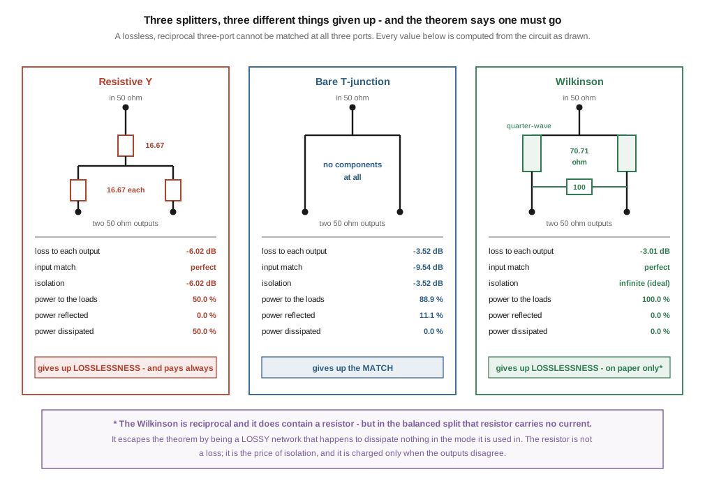
This volume establishes the framework the rest of the dive uses, and it does so from a single structural result: a three-port network cannot simultaneously be lossless, reciprocal, and matched at all three ports. That is not a rule of thumb or an engineering approximation; it follows in three lines from the unitarity of a lossless scattering matrix, and no amount of cleverness evades it. Every passive splitter in existence is a choice about which of those three properties to surrender, and the three topologies in the lead figure are the three available answers.

Two conclusions from this volume run against what is usually written, and both are worth stating at the top rather than leaving the reader to find them.

The first is that the resistive divider’s isolation is not zero. The previous edition of this chapter stated that a resistive splitter offers “~0 dB” of isolation between its outputs, and listed that as its defining weakness beside its 6 dB loss. Section 3 computes the network exactly and finds the isolation is 6.02 dB — identical to its insertion loss, and for the same reason. Six decibels is poor isolation and the chapter’s practical advice survives unchanged, but zero and six are different numbers, and the second one turns out to explain the device.

The second is that a splitter with no resistor in it is exactly lossless. The previous edition listed “splitter with no resistor is lossless” as a myth to be dispelled. Section 4 computes the bare junction and finds it dissipates nothing whatever: 88.89 % of the input power reaches the two loads and the remaining 11.11 % is reflected back to the source, summing to unity to the last digit. The junction is a bad splitter, but not because it wastes power. It is a bad splitter because it is unmatched and because its outputs are coupled to each other at 3.52 dB — and “reflected” and “dissipated” are not interchangeable words when the thing doing the reflecting is connected to a transmitter.

The two corrections have the same shape, and it is the shape this dive keeps finding: the conclusion in the seed chapter is usually right, and the mechanism attached to it is usually wrong. That matters more than it sounds, because a reader who has the right answer for the wrong reason cannot extrapolate. The rest of this dive is largely an exercise in reattaching conclusions to the mechanisms that actually produce them.

1.2 The theorem that governs every splitter ever built

Take a three-port network and ask for three reasonable things at once. Ask that it be matched at every port, so that a signal arriving at any port sees 50 Ω and nothing bounces. Ask that it be reciprocal, which any network built from ordinary passive components — resistors, inductors, capacitors, transmission lines — necessarily is. And ask that it be lossless, so that all the power going in comes out somewhere useful.

Write the scattering matrix. Matched at all ports means the diagonal is zero. Reciprocal means the matrix equals its own transpose. Lossless means the matrix is unitary: every column has unit magnitude and every pair of distinct columns is orthogonal.

The three conditions collide immediately. Orthogonality of the first two columns, with the diagonal zeroed, reduces to the requirement that S₁₃* S₂₃ = 0 — so at least one of S₁₃ and S₂₃ must vanish. Repeating the argument on the other two column pairs forces at least two of the three off-diagonal terms to vanish. A network with two of its three couplings equal to zero is not a splitter; it is a two-port with an orphan port bolted to the side of it.

So the three requirements are jointly unsatisfiable, and any real device gives one up:

• Give up losslessness and you get the resistive divider, which is matched and reciprocal and turns half its input into heat, every time, regardless of what the loads are doing.
• Give up the match and you get the bare junction, which is lossless and reciprocal and reflects 11 % of what you feed it.
• Give up losslessness, but only nominally, and you get the Wilkinson — a network that formally contains a resistor, and therefore formally escapes the theorem, but which arranges for that resistor to carry no current at all when the outputs are behaving. It is matched at every port, it delivers 100 % of the input power to the loads, and its isolation is infinite at the design frequency. On paper it pays the theorem’s price. In practice it pays nothing.

That third line is the reason the Wilkinson is the canonical splitter and the reason Vol 2 is devoted to it. It is worth being precise about what the escape is and is not. The Wilkinson does not violate the theorem; a lossless network is one whose scattering matrix is unitary, and the Wilkinson’s is not, because a resistor is present and some excitations of the network do dissipate power in it. What the Wilkinson achieves is that the particular excitation an operator cares about — one input, two equal in-phase outputs, everything terminated — is not one of them.

There is a fourth escape, and it is the subject of Vol 3: stop building a three-port. The theorem says nothing about four-port networks, and a four-port can be simultaneously lossless, reciprocal and matched at all ports — which is exactly what a branch-line hybrid, a rat-race and a coupled-line coupler each are. The price is the fourth port, which has to be there and has to be terminated, and the reward is that phase becomes a design variable rather than an accident.

1.3 The resistive divider, derived rather than quoted

The simplest splitter is three equal resistors in a Y. For a 50 Ω system each is Z₀/3 = 16.67 Ω, and the value is not arbitrary: it is the only value that matches all three ports simultaneously.

Check that first, because it is the property the resistors are bought for. Looking into port 1 with ports 2 and 3 terminated in 50 Ω, the path is one 16.67 Ω resistor in series with the parallel combination of the two output branches, each of which is 16.67 + 50 = 66.67 Ω:

Z_in = 16.67 + (66.67 ‖ 66.67) = 16.67 + 33.33 = 50.00 Ω

Exactly 50, with no approximation anywhere. By symmetry the same holds at every port, so the network is matched at all three — which is the first of the theorem’s three properties, bought and paid for.

Now the transmission. With a unit voltage at the port-1 terminal, the junction node sits at 33.33 / 50 = 0.6667, and each output load takes 50 / 66.67 of that:

S₂₁ = S₃₁ = 0.6667 × 0.75 = 0.5000 exactly, which is −6.02 dB.

Half the voltage is a quarter of the power, so each load receives 25 % of the input and the two together receive 50 %. The other 50 % is dissipated in the resistors, and there is nowhere else for it to be, since nothing is reflected. That is the second of the three properties, surrendered.

The seed chapter’s headline number — 6 dB per output rather than 3 — is therefore confirmed exactly, and so is its decomposition into “3 dB inherent split loss plus 3 dB resistive dissipation”. Half the power is thrown away and the surviving half is divided in two; both halvings are 3.01 dB and they compound to 6.02. That reading is correct and should not be re-opened by a later pass.

What is not correct is the explanation the chapter attaches to it. Its §3.3 says the second 3 dB arises because “the resistor network drops the impedance from 50/2 = 25 Ω back up to 50 Ω at each output”. No such operation occurs. There is no 25 Ω anywhere in the analysis, nothing is being transformed, and the sentence describes a matching network rather than the divider it is about. The actual mechanism is the voltage division computed above, and it is both simpler and more useful: the resistive divider loses 6 dB because its transmission coefficient is one half in voltage, and a factor of two in voltage is a factor of four in power.

1.3.1 The isolation is 6.02 dB, not zero

The chapter’s other claim about this network is that its isolation is approximately zero — that the resistors do nothing to decouple the outputs from one another. This is the claim that does not survive computation, and the correction is pleasing because it needs no new arithmetic.

Drive port 2 instead of port 1, with ports 1 and 3 terminated. The network is symmetric under exchange of any two ports, so the calculation is character-for-character the one already done:

S₃₂ = 0.5000, i.e. −6.02 dB.

The isolation between the two outputs is 6.02 dB — numerically identical to the insertion loss, and identical for the structural reason that in a fully symmetric network every port looks like every other. Six decibels is genuinely poor; it means a signal re-radiated from one receiver’s front end arrives at the other attenuated only fourfold in power, which is why the chapter’s practical guidance to avoid this topology where isolation matters is sound. But the specific figure matters when a reader is comparing options. Against a Wilkinson’s 20–25 dB in a real part, a resistive divider is roughly 15 to 19 dB worse — not infinitely worse — and for a bench setup feeding two well-matched instruments that can be an acceptable trade for DC-to-daylight bandwidth.

This is worth flagging as a pattern rather than an isolated slip. “Approximately zero” is what isolation feels like in a device with no isolating element in it, and the chapter reached for the intuitive figure instead of the computed one. The same substitution shows up again in Vol 2’s bandwidth figures and in Vol 4’s account of directivity.

1.3.2 What the resistive divider is actually for

Given 6 dB of loss and 6 dB of isolation, the case for this topology rests entirely on the two things it does better than anything else: bandwidth and predictability.

The analysis above contains no frequency term. There is no transmission line, no resonance, no reactance, and therefore no band edges — a resistive divider works from DC to the frequency at which its own parasitic inductance and capacitance stop being negligible, which for a well-built surface-mount part is several gigahertz. Nothing else in this dive comes close. The Wilkinson of Vol 2 is a quarter-wave structure and is confined to a band around its design frequency; the transformer splitters are bounded below by core permeability and above by leakage inductance; the hybrids of Vol 3 are narrower still.

It also has a flat, unconditional 6 dB. The loss does not vary with frequency, with load mismatch, or with what the other output is connected to, which makes a resistive divider the right instrument for a measurement setup where a known, constant, frequency-independent attenuation is worth more than 3 dB of signal. Its power handling is set by the resistors and is genuinely low — the chapter’s “2–10 W for amateur use” is a fair characterisation, bearing in mind that under a fault condition a single resistor can be asked to take a large fraction of the input.

1.4 The bare junction is lossless, and that is not enough

The chapter’s list of myths includes this one: “Splitter with no resistor is lossless — false in the passive case. T-junctions without a Wilkinson resistor have 0 dB isolation and 100 % reflective interaction between branches; the resulting standing-wave pattern wastes power and corrupts both outputs.”

The conclusion — do not do this — is right. Every other clause is wrong, and the computation takes one line.

A bare three-way junction is two 50 Ω loads in parallel presented to a 50 Ω source, so the input sees 25 Ω:

S₁₁ = (25 − 50)/(25 + 50) = −1/3, a return loss of 9.54 dB, an SWR of 2.00:1

S₂₁ = S₃₁ = 1 + S₁₁ = 2/3, i.e. −3.52 dB

Now account for the power. Each output takes (2/3)² = 44.44 %, the two together take 88.89 %, and the reflection carries (1/3)² = 11.11 %. The sum is 100.00 %. Nothing is dissipated, because there is nothing in the circuit capable of dissipating anything — the network is three wires meeting at a point.

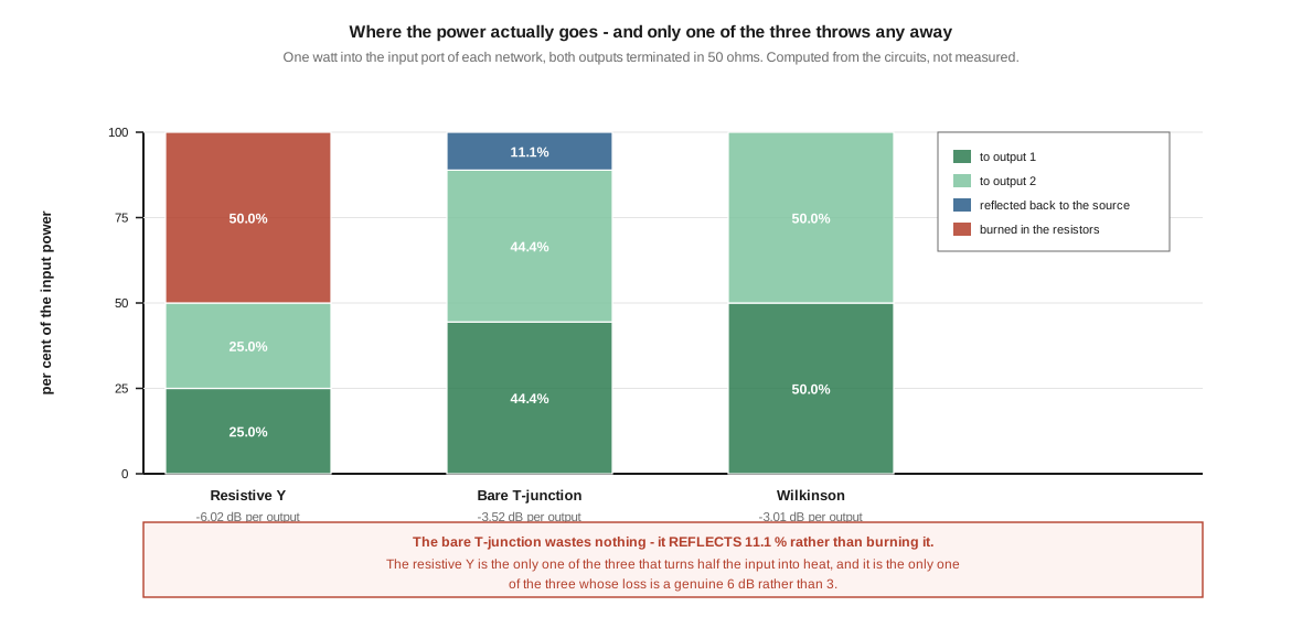
So the bare junction is lossless, has an isolation of 3.52 dB rather than 0 dB, and its 11.11 % shortfall is returned to the source rather than wasted. The distinction between reflected and dissipated is not pedantry. Power that is dissipated is gone. Power that is reflected goes back down the feedline to the transmitter, where it adds to or subtracts from the forward wave depending on line length, shows up on an SWR meter, and in a solid-state final may trigger foldback. A device that reflects 11 % of a kilowatt is doing something a device that absorbs 11 % of a kilowatt is not.

Two further points fall out of the same three numbers, and both are useful later.

The junction sits between the other two on loss, and its entire excess is the reflection. The Wilkinson delivers 3.01 dB per output, the theoretical floor for a two-way division; the bare junction delivers 3.52 dB; the resistive divider delivers 6.02 dB. The junction’s 0.51 dB of excess over the floor is exactly the 11.11 % that came back out of the input port — 10·log₁₀(1 / 0.8889) = 0.51 dB — and nothing else. Remove the quarter-wave transformers from a Wilkinson and this is precisely what remains: the same three conductors meeting at a point, with the impedance transformation that produced the input match taken away.

And the junction’s isolation and its insertion loss are again the same number, 3.52 dB, for the same symmetry reason as in §3.1. In any three-port with no isolating element, a signal entering one output port sees the other output port exactly as the input port would. Isolation is not a property that can be added later; it has to be designed in, and the only way to design it in is to give the network somewhere for the difference between the two outputs to go.

1.5 The Wilkinson’s escape — a resistor that dissipates nothing

Ernest Wilkinson’s answer, published in the IRE Transactions on Microwave Theory and Techniques in 1960, is to take the bare junction, insert a quarter-wave transformer in each branch, and bridge the two outputs with a resistor. Vol 2 derives the whole thing properly. What matters here is the structural point, which is the spine of this dive.

The two branch lines have a characteristic impedance of Z₀√2 = 70.71 Ω. Each transforms its 50 Ω load to 70.71²/50 = 100 Ω at the input node, and two 100 Ω branches in parallel are 50 Ω — so the input is matched exactly, with no reflection at all. Each output receives half the power: S₂₁ = S₃₁ = 1/√2, which is −3.01 dB, the theoretical minimum for a two-way division. The bridging resistor is 2Z₀ = 100 Ω.

And in that condition the resistor carries no current. Both of its terminals sit at the same voltage, because the two branches are identical and are driven identically, so the potential difference across it is zero. It might as well not be fitted. All the input power reaches the loads; the network is matched at every port; the isolation between the outputs is infinite at the design frequency. Three for three, from a network that formally surrendered losslessness in order to be allowed to exist.

The resistor’s value is not arbitrary either, and it is worth separating from a coincidence the seed chapter builds an explanation on. Its §4.2 states that the 70.71 Ω line impedance is “the geometric mean of the input (50 Ω) and the bridging resistor (100 Ω)”. It is true that √(50 × 100) = 70.71, and it is true that the bridging resistor is 100 Ω, but the relationship is coincidental rather than causal. The line impedance is fixed by the requirement that each of two parallel branches present 100 Ω at the input, which is a statement about 2Z₀ and has nothing to do with the resistor; the resistor is fixed independently, by the odd-mode analysis in Vol 2, which also lands on 2Z₀. Two different derivations arriving at the same number is not one derivation. The chapter’s own §4.2 then admits the confusion in print — “the impedance match math is more complex than this simplified explanation captures” — which is an honest sentence in the wrong place. The derivation is not complex; it is one line, and Vol 2 gives it.

The seed also attributes the Wilkinson’s excess loss to the resistor: “3 dB inherent + ~0.3–0.5 dB resistive”. The resistive element contributes nothing to the loss of a balanced split, as just shown. Real Wilkinson dividers do show a few tenths of a decibel of excess loss, and it is conductor and dielectric loss in the quarter-wave lines — which is why it scales with line length, why it is worse on FR-4 than on PTFE, and why the multi-section designs of Vol 2 that buy bandwidth by adding sections pay for it in exactly that coin. Calling it resistive loss attaches a real number to the wrong component and predicts the wrong scaling.

1.6 Splitter and combiner are one device, and the resistor is where they differ

Every passive splitter is reciprocal, so the same box run backwards combines. The seed says so, and it is right; this is one of the claims in the chapter that needs no correction at all. The subtlety — which the chapter also gets right, and which is worth quantifying because it is the single most practically important number in this volume — is what happens to the isolation resistor when it is used that way.

Feed two equal-amplitude signals into the two output ports of a Wilkinson and take the sum from the input port. Decompose them into an even part, which is their average, and an odd part, which is half their difference. The even part sees the network exactly as in §5: it passes to the sum port, and the resistor is invisible to it. The odd part sees a virtual short at the centre of the network and terminates entirely in the resistor. The sum goes to the load and the difference goes to the resistor, and there is no third destination.

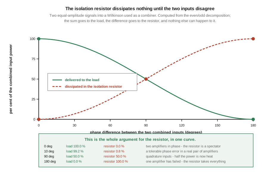
For two equal-amplitude inputs differing in phase by φ, the fraction reaching the load is cos²(φ/2):

Table 1 — For two equal-amplitude inputs differing in phase by φ, the fraction reaching the load is cos²(φ/2)

phase difference	to the load	into the resistor
0°	100.00 %	0.00 %
10°	99.24 %	0.76 %
30°	93.30 %	6.70 %
60°	75.00 %	25.00 %
90°	50.00 %	50.00 %
120°	25.00 %	75.00 %
180°	0.00 %	100.00 %

Amplitude imbalance is far more forgiving than phase error, which is not obvious in advance. Two in-phase inputs differing by 1.0 dB in amplitude still deliver 99.67 % to the load and put only 0.33 % into the resistor; even a 3.0 dB imbalance delivers 97.16 %. A 30° phase error, by contrast, costs twenty times as much as a 1 dB amplitude error. In a combined pair of amplifiers, phase tracking is the specification to worry about and gain matching is comparatively cheap.

Three practical consequences follow, and they are the reason this section exists.

A combiner’s resistor must be rated for the failure, not for the operation. In normal service it dissipates a fraction of a per cent. If one of two combined amplifiers fails, the phase difference is irrelevant — the surviving amplifier’s power divides equally between the load and the resistor, so the resistor takes half of the surviving amplifier’s output. A pair of 500 W amplifiers combining into 1 kW needs an isolation resistor capable of 250 W to survive a single-amplifier failure, and this is precisely why commercial high-power combiners carry resistors that look absurdly oversized for a device advertised as low-loss.

The resistor is an instrument. Its dissipation is a direct, continuous measurement of how badly the two inputs disagree. Monitoring the temperature of the isolation resistor in a combined pair is the standard way of detecting a developing imbalance before it becomes a failure, and it works because the resistor sees the difference signal and nothing else.

And the 3 dB question resolves cleanly. The seed says that combining two amplifiers gives “0 dB increase in output power per amplifier but +3 dB total over a single amp’s output”. That is correct as stated and should not be changed. Two 100 W amplifiers combined in phase deliver 200 W, which is 3.01 dB above 100 W, with no loss in the combining process — the transformers are lossless and the resistor is a spectator. The combining operation itself is free; it is the phase discipline that costs, and the table above is the price list.

1.7 What isolation is actually for

Isolation is the specification most often quoted about splitters and least often connected to a consequence. It is worth stating what it buys, because the answer depends on which direction the splitter is being used in, and the two cases have almost nothing to do with each other.

On receive, splitting one antenna among several receivers, isolation controls how much of what each receiver emits reaches the others. Every superheterodyne receiver leaks local-oscillator energy back out of its antenna port; a direct-sampling SDR leaks clock harmonics and switching noise. With 6 dB of isolation, a −40 dBm LO leak from one receiver arrives at the next at −46 dBm, which is an enormous signal by HF standards and will appear as a birdie that moves when the other operator tunes. With 25 dB it arrives at −65 dBm, which is still detectable but is usually below the external noise floor that the receive-loop dive establishes for any real site. This is the dominant reason to want isolation in a receive distribution system, and it is not about signal loss at all.

On transmit, combining several sources into one antenna, isolation controls how much of each amplifier’s output is delivered into the other amplifier’s output stage. This is a much harsher requirement, because the quantity involved is not a leak but a substantial fraction of full power, and the consequence is not a birdie but a destroyed output device.

And in a measurement setup, isolation controls whether the instrument is measuring the device or measuring the other instrument. The NanoVNA dive makes the general point: the quantity a VNA reports is a ratio, and a ratio is only meaningful if the reference path is genuinely independent of the measurement path.

What isolation is not is a proxy for quality. A resistive divider with 6 dB of isolation is the right component for a wideband bench setup where the two outputs go to a spectrum analyser and an oscilloscope, neither of which emits anything. A 25 dB Wilkinson is the wrong component if the required band is 10 MHz to 6 GHz, because it cannot cover it. Vol 2 quantifies exactly how narrow a single-section Wilkinson is, and the answer depends entirely on what threshold is being demanded of it — which turns out to be the other variable the seed chapter’s tables leave out.

1.8 Where this volume hands off

The framework is in place. A three-port splitter cannot be matched, lossless and reciprocal at once, and the three real topologies are the three ways of surrendering one of those. The resistive divider surrenders losslessness unconditionally and pays 6.02 dB for it, with 6.02 dB of isolation into the bargain rather than the zero usually quoted — but it pays that price flat from DC to microwave, which nothing else in this dive can offer. The bare junction surrenders the match, and is exactly lossless while being useless: its 11.11 % deficit is reflected rather than dissipated, and its outputs are coupled at 3.52 dB. The Wilkinson surrenders losslessness formally and nothing at all in practice, because its resistor carries no current when the outputs agree — and when they disagree, it takes the entire difference, which is what makes it both an isolator and a diagnostic.

From here:

• Vol 2 — The Wilkinson, and the resistor that dissipates nothing derives the even/odd-mode analysis properly, computes the bandwidth against a stated threshold rather than quoting a bare percentage, and settles the N-way question — where the seed’s own table and its own DIY build contradict each other about whether a four-way splitter is a star or a tree. It also covers the ferrite transformer realisation that carries the whole of HF, where a quarter-wave line is measured in tens of metres.
• Vol 3 — Four ports, and what the phase buys takes the fourth escape from §2’s theorem: the branch-line hybrid, the rat-race and the coupled-line coupler, which achieve simultaneously what no three-port can. It computes each one’s bandwidth and phase error across the band, and corrects the seed’s account of the rat-race’s geometry, which is internally inconsistent as printed.
• Vol 4 — Sampling instead of splitting is about the directional coupler, the device that deliberately divides unequally in order to measure. Directivity is the specification that matters and the one the chapter treats loosely; Vol 4 turns it into an error bar on an SWR reading. It also settles what is inside a NanoVNA, where the seed chapter and this hub’s own NanoVNA dive currently disagree.
• Vol 5 — DIY build, measurement and buys builds a Wilkinson correctly — the seed’s PCB dimensions are self-contradictory and the design it specifies will not fit on the board it specifies — measures it on a VNA, and surveys what can actually be bought. That survey has real work to do: of the manufacturer part numbers checked so far, every single one had its frequency range stated wrongly.

One limitation is recorded rather than skipped. Every figure in this volume is computed from an idealised circuit — perfect resistors, lossless lines, ideal terminations. Real components have parasitic reactance, real lines have loss, and real terminations are not 50 + j0. The idealisations are appropriate here because the volume’s subject is what is structurally possible rather than what a particular part achieves, but none of these numbers is a measurement, and Vol 5 §4 is written as the bench procedure that would turn them into one.

1.9 Resources

• E. J. Wilkinson, An N-Way Hybrid Power Divider, IRE Transactions on Microwave Theory and Techniques, vol. 8, no. 1, pp. 116–118, 1960 — the original paper. Its abstract describes a circularly symmetric divider giving “isolation between output terminals and approximately matched terminal impedances over about a 20 per cent band”, a figure Vol 2 reproduces independently and pins to a specific threshold.
• D. M. Pozar, Microwave Engineering, 4th ed., ch. 7 — the canonical treatment of power dividers and directional couplers, and the source of the three-port argument in §2 in its standard form.
• BALUNs and UNUNs, Vol 1 — transmission-line transformers, the technology the HF splitters of Vol 2 are built from.
• Antenna tuners, Vol 1 — impedance transformation by variable-ratio networks, and the companion discussion of what a matching network can and cannot reach.
• NanoVNA, Vol 1 — the reflection coefficient as the primitive quantity, and the instrument used to verify everything in Vol 5.
• Receive-only loops, Vol 1 — the external-noise floor that decides whether a splitter’s 6 dB matters at all on receive.
• Active splitters and distribution amplifiers — the other half of the distribution problem, for the cases where the loss computed here cannot be absorbed.