Sampling Instead of Splitting

---

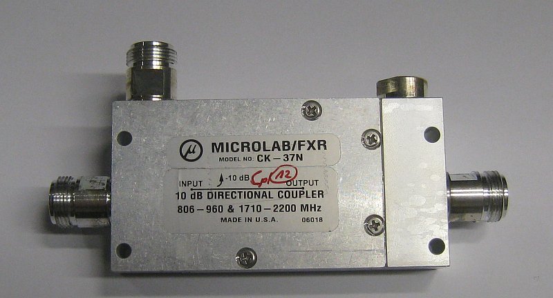
4.1 About this volume

The first three volumes were about dividing power so that the outputs are equal. This one is about dividing it so that they are deliberately, precisely unequal — because the purpose is no longer distribution but measurement.

A directional coupler is the same four-port structure Vol 3 analysed, operated with a loose coupling factor so that the main path is barely disturbed while a small, accurately-known sample is extracted. What makes it an instrument rather than a lossy splitter is that the sample is taken from waves travelling in one direction only. That property is the whole device, and the specification that measures it — directivity — is the one the seed chapter treats most loosely.

This volume’s argument is that directivity is not a quality score; it is the error bar on every reading the instrument produces, and that once it is written that way a great deal of received wisdom about SWR meters becomes quantitative. §3 computes it.

Two corrections are worth stating at the top.

The chapter’s accuracy claim for a 30 dB coupler is wrong, and by a useful amount. It says 30 dB of directivity is “adequate for SWR measurements down to 1.1:1 accuracy”. Computed, a coupler with 30 dB of directivity presented with a true 1.10:1 load can legitimately read anywhere from 1.03:1 to 1.17:1. The uncertainty is not 1.1:1; at 1.1:1 the uncertainty is most of the interesting range.

And the chapter says a NanoVNA contains two directional couplers. It does not, and this hub’s own NanoVNA dive already says so in terms — a resistive bridge, with the physical reason given. §5 settles the contradiction, which is the first time in this program that two dives in the same hub have been found asserting incompatible things about the same hardware.

4.2 Three specifications, and only one of them is hard

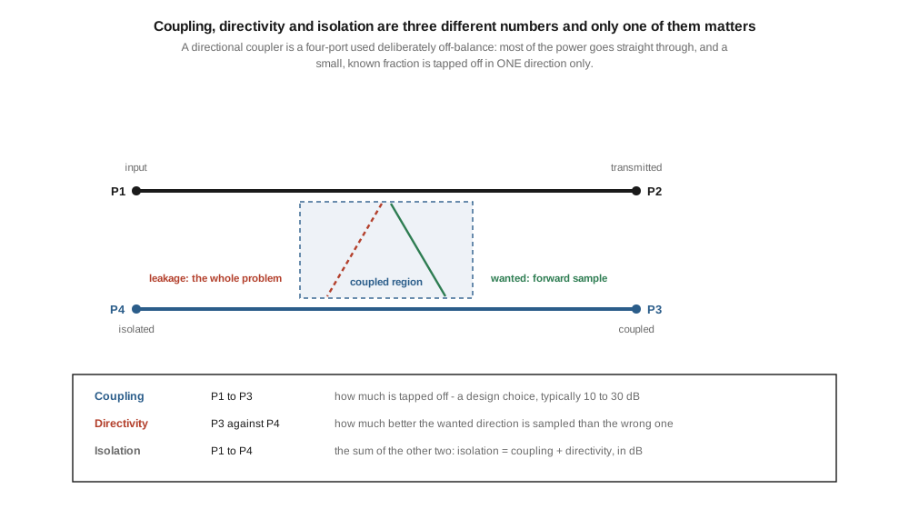
A directional coupler has four ports. Power enters P1 and leaves almost entirely at P2. A small fraction appears at P3, the coupled port. Ideally nothing at all appears at P4, the isolated port, which is terminated — and in most commercial couplers that termination is inside the case, which is why a device with four ports is sold with three connectors.

Three numbers describe it, and the chapter lists all three correctly:

Coupling is the ratio of P3 to P1, typically 10 to 30 dB. It is a design choice, set by the geometry — Vol 3 §8 gives the even and odd mode impedances required for each value — and it is not difficult to hit.

Directivity is the ratio of what appears at the coupled port for a forward wave to what appears there for an identical reverse wave. It is the measure of how well the device distinguishes direction, and it is entirely a question of how perfectly the structure’s symmetry and termination are realised. This is the hard one.

Isolation is the ratio of P4 to P1, and the chapter’s relation is exactly right: isolation = coupling + directivity, in decibels. Confirmed, not corrected. A 20 dB coupler with 30 dB directivity has 50 dB isolation. The relation is definitional rather than empirical, which is why it holds exactly, and it is the reason the three numbers are never independently specified — quoting any two fixes the third.

The chapter’s separate myth-list entry on this point is also right and worth keeping: “Directivity = isolation — distinct specs.” They are, and the distinction is that directivity is referenced to the coupled port while isolation is referenced to the input.

One further relation, which the chapter states confusingly in its myths and which is worth having cleanly. In a lossless coupler the main path loses exactly the power the coupled port removes:

through-path loss = 10·log₁₀(1 − c²), where c = 10^(−C/20)

A 20 dB coupler takes 1 % of the power and costs the main path 0.04 dB. A 10 dB coupler takes 10 % and costs 0.46 dB. A 3 dB coupler takes half and costs 3.02 dB. The chapter’s §8.2 gives a directional coupler’s insertion loss as “0.2–0.5 dB”, which is a reasonable figure for a real 10 to 20 dB coupler once conductor loss is included, but it presents it as an independent specification when most of it, for tighter couplings, is simply the coupled power leaving. A coupler’s main-path loss is not a defect; for the most part it is the measurement.

4.3 Directivity is the error bar

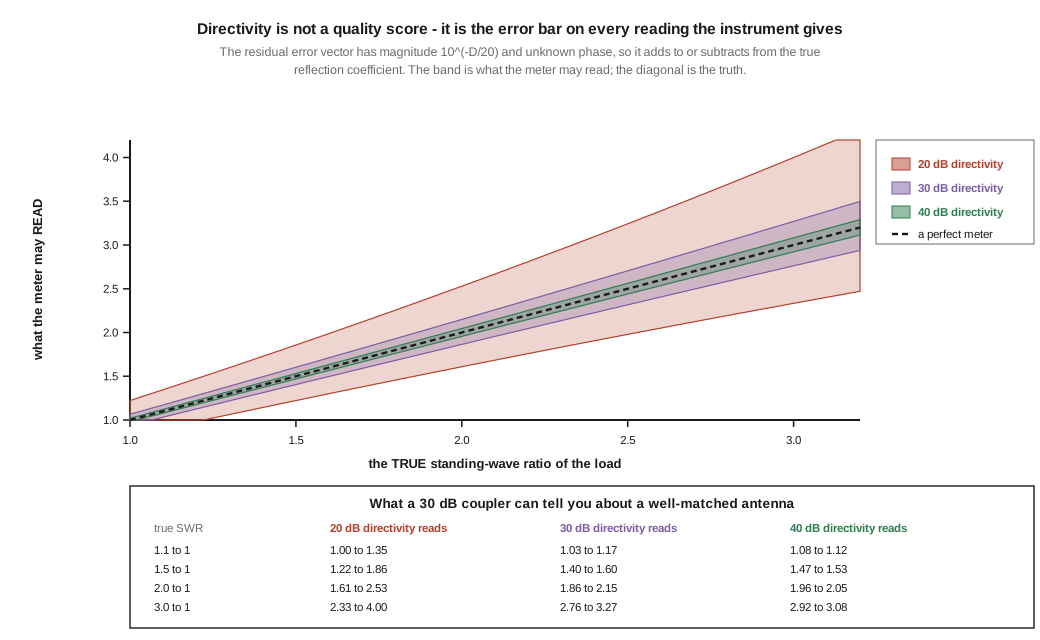
Here is the mechanism, and it is short. A coupler with directivity D decibels leaks a residual of the reverse wave into the forward sample (and vice versa) with relative magnitude d = 10^(−D/20). Its phase is unknown — it depends on the cable length, the connector, the frequency, everything the calibration did not capture. So a measurement of a true reflection coefficient ρ returns some value between ρ − d and ρ + d, and every value in that interval is equally consistent with the instrument.

Converting to SWR:

Table 1 — Converting to SWR

true SWR	20 dB directivity reads	30 dB directivity reads	40 dB directivity reads
1.10 : 1	1.00 to 1.35	1.03 to 1.17	1.08 to 1.12
1.50 : 1	1.22 to 1.86	1.41 to 1.60	1.47 to 1.53
2.00 : 1	1.61 to 2.53	1.86 to 2.15	1.96 to 2.05
3.00 : 1	2.33 to 4.00	2.76 to 3.27	2.92 to 3.08

The chapter’s claim that 30 dB is “adequate for SWR measurements down to 1.1:1 accuracy” is the entry to correct. At 30 dB of directivity a genuinely 1.10:1 antenna reads somewhere between 1.03 and 1.17. The instrument cannot distinguish a 1.03:1 antenna from a 1.17:1 antenna, and both of those are perfectly good antennas, so the reading carries almost no information at that end of the scale.

Three consequences follow, and they are the practical content of this volume.

The error is worst, in fractional terms, where the match is best. At 3:1 a 30 dB coupler is accurate to about ±8 %; at 1.1:1 it is accurate to about ±60 % of the excess SWR above unity. This inverts the usual intuition that a good match is easy to measure. It is the hardest thing to measure, because the quantity being measured is small and the error is fixed in absolute terms.

A 20 dB coupler cannot certify a good antenna at all. At 20 dB directivity a true 1.10:1 load can read as 1.00:1 — a perfect match, on an antenna that is not perfectly matched. Any SWR meter reporting exactly 1.0:1 should be read as “below the directivity floor of this instrument”, never as a measurement.

And this is exactly why a VNA is calibrated. Directivity is a systematic, repeatable error, not noise. The whole purpose of the open/short/load sequence that the NanoVNA dive describes is to measure the residual directivity error term and subtract it arithmetically. A calibrated instrument’s effective directivity is far better than its raw hardware directivity — which is the single strongest argument for using a calibrated VNA rather than an SWR meter to evaluate an antenna that is already close to matched.

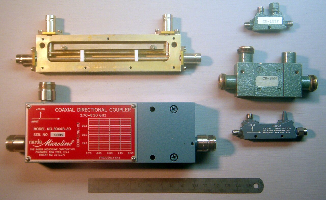
The chapter’s own statement that good couplers achieve “30+ dB directivity” is fair, and the Narda unit visible in the photograph below carries a printed coupling-versus-frequency chart on its case precisely because these are instruments whose small deviations are worth documenting per unit.

4.4 What a coupler is made of

At VHF and above, a directional coupler is the coupled-line structure of Vol 3 §8: two transmission lines run parallel over a quarter wavelength, with the coupling set by the gap. At 20 dB the required even/odd impedance ratio is 1.22, which two ordinary parallel traces provide, and this is why loose couplers are cheap and ubiquitous.

Below VHF the quarter-wave requirement bites exactly as it did for the Wilkinson in Vol 2 §8, and the answer is the same: a transformer. A current transformer sampling the line current and a capacitive divider sampling the line voltage produce two samples whose sum is proportional to the forward wave and whose difference is proportional to the reflected wave. Combine them one way and the reverse wave cancels; combine them the other and the forward wave does. This is the classic Bruene coupler, and it is what is inside essentially every amateur HF SWR meter.

Two things follow that the chapter does not draw out.

The directivity of a Bruene coupler depends on a balance between a transformer and a capacitor, which is why these instruments have an internal trimmer and why their directivity degrades away from the frequency at which it was set. This is the mechanism behind a familiar complaint — that an HF SWR meter reads differently on 10 m than on 80 m into the same load — and it is a directivity problem, not a calibration drift.

And the Bird 43 is exactly this, made rotatable. The chapter’s §8.1 says “A Bird wattmeter has a coupler inside that samples the forward (or reflected) wave”, and that is correct and confirmed. The instrument’s removable slug contains the coupling element, and rotating the slug through 180° physically reverses the sampled direction — which is why a Bird reads forward and reflected by being turned around rather than by a switch, and why each slug covers one band and one power range: the coupling factor and the frequency response are properties of that particular element.

4.5 The bridge that is not a coupler

The chapter’s §8.3 says:

The NanoVNA’s reflection bridge uses two directional couplers plus a reference oscillator. […] The NanoVNA’s directional couplers are PCB-embedded with directivity of ~35 dB across 100 MHz – 1.5 GHz.

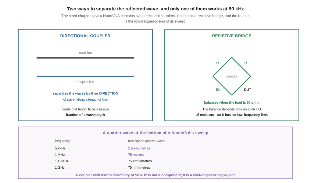
The first sentence contradicts itself — a bridge is named in the subject and couplers in the predicate — and it contradicts this hub’s own NanoVNA dive, which states plainly that the front end is “a resistive bridge, not a directional coupler” and gives the reason.

The reason is decisive and can be put in one table. A coupled-line directional coupler separates waves by their direction of travel along a length of line, and needs that length to be a usable fraction of a wavelength. The free-space quarter wave is:

Table 2 — The reason is decisive and can be put in one table. A coupled-line directional coupler separates waves by their direction of travel along a length of line, and needs that length to be a usable fraction of a wavelength. The free-space quarter wave is

frequency	quarter wave
50 kHz	1.5 kilometres
1 MHz	75 metres
100 MHz	750 millimetres
1 GHz	75 millimetres

A NanoVNA sweeps from tens of kilohertz. A coupler with useful directivity at the bottom of that sweep is not a component that fits in a handheld instrument, and no amount of PCB cleverness changes the wavelength of a 50 kHz wave.

A resistive bridge has no such limit, because its balance condition depends only on the ratio of its resistor arms and not on any physical length. Four arms, one of them the unknown; when the unknown equals Z₀ the bridge balances and the detector sees nothing; any mismatch unbalances it by an amount proportional to Γ. That works from DC upward, and it fails only at the high end where the resistors stop being resistive.

So the bridge is the correct answer, and the correction runs in the direction the NanoVNA dive already had it. Two further points belong with it.

The chapter’s “~35 dB across 100 MHz – 1.5 GHz” figure is withdrawn rather than restated. No source could be found for it in this pass, it is attached to hardware that is not what the instrument contains, and a plausible-looking number with no provenance is precisely what this program has learned to remove rather than soften. What can be said without a source is structural: a resistive bridge’s raw directivity is modest by laboratory standards, and the open/short/load calibration exists to characterise and subtract it.

And the trade is real in both directions. A laboratory VNA working above a gigahertz does use directional couplers, because at those frequencies a coupler is small, its directivity is excellent, and it does not have a bridge’s insertion loss. The right statement is not that bridges are better than couplers but that the choice is set by the low end of the required sweep. §3’s argument about calibration applies to either.

4.6 The bias-T is two components and two inequalities

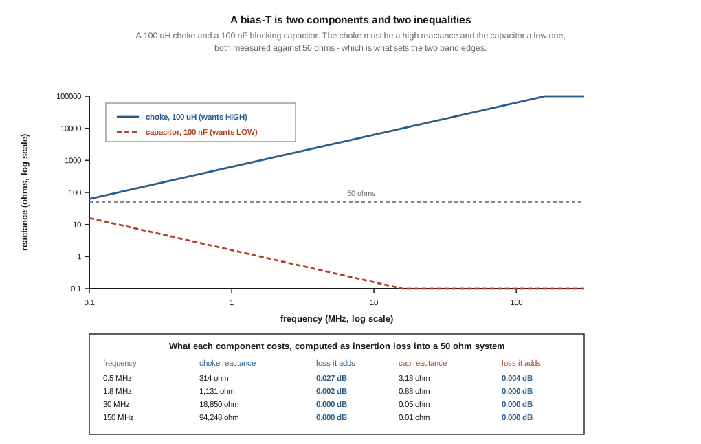
A bias-T is not really a member of the coupler family; it divides RF from DC rather than dividing RF from itself. It earns a place here because it is what makes a masthead amplifier possible, and because the chapter’s account of it contains an inverted statement.

The principle the chapter gives is correct and is confirmed: “a capacitor passes RF and blocks DC; an inductor passes DC and blocks RF”. What it does not give is the quantitative form, which is two inequalities against the system impedance:

• the series blocking capacitor must have X_C ≪ Z₀, so it does not attenuate the signal
• the shunt feed choke must have X_L ≫ Z₀, so it does not shunt the signal away

Computing both for a 100 µH choke and a 100 nF capacitor in a 50 Ω system:

Table 3 — Computing both for a 100 µH choke and a 100 nF capacitor in a 50 Ω system

frequency	choke reactance	loss it adds	capacitor reactance	loss it adds
0.5 MHz	314 Ω	0.027 dB	3.18 Ω	0.004 dB
1.8 MHz	1 131 Ω	0.002 dB	0.88 Ω	0.000 dB
30 MHz	18 850 Ω	0.000 dB	0.05 Ω	0.000 dB
150 MHz	94 248 Ω	0.000 dB	0.01 Ω	0.000 dB

Those two ordinary components are effectively lossless across the whole of HF and well into VHF. The low-frequency edge is where the inequalities fail: the choke’s reactance falls to 50 Ω at about 80 kHz and the capacitor’s rises to 50 Ω at about 32 kHz, and below that the device stops working in both senses at once.

The chapter’s myth entry on this is half inverted. It says: “Outside the band, the capacitor’s reactance changes (lower at low f) and the inductor’s reactance changes (higher at high f) — the separation degrades.” The inductor clause is right. The capacitor clause is backwards: X_C = 1/(2πfC) is higher at low frequency, which is exactly why a blocking capacitor fails at the bottom of the band and not the top. As written the sentence describes a capacitor that gets better as the frequency falls, which would mean a bias-T has no low-frequency limit at all — and the table above shows that it does.

A caveat belongs with the table, and it is the thing that actually limits real bias-Ts. Both components above are ideal. A real 100 µH choke has self-capacitance and therefore a self-resonant frequency, above which it behaves as a capacitor and stops choking; a real capacitor has series inductance and its own self-resonance, above which it stops passing. The upper limit of a practical bias-T is set by those parasitics, not by the reactances computed here, which is why wideband commercial bias-Ts use several staggered components rather than one of each. The chapter’s own observation that the RF range extends to gigahertz “wider with multi-element designs” is therefore right, and this is the mechanism behind it.

4.7 The gotchas, weighed

The chapter closes with a list of myths. Several are sound and deserve to be confirmed rather than quietly re-derived, since over-correction is a named failure mode in this program.

Confirmed as stated: that directivity and isolation are distinct specifications; that isolation = coupling + directivity; that a Bird wattmeter contains a coupler; that higher coupling does not mean a better coupler, the right coupling being application-dependent; and the distinction between crossed-needle meters that display forward and reflected simultaneously and single-needle meters that switch between them.

Corrected: the bias-T’s capacitor reactance, inverted in §6; the 30 dB directivity accuracy claim, quantified in §3; and the NanoVNA’s front end, settled in §5.

Sharpened rather than corrected: the entry claiming coupling and insertion loss are related. They are, but the clean statement is the 10·log₁₀(1 − c²) of §2, which makes it an identity rather than a tendency.

One entry deserves a longer answer than the chapter gives it, because it is the one that costs people money. “Cheap eBay splitters with no published S-parameters — the specs are usually wishful thinking.” The useful form of that advice is a test rather than a warning, and §3 supplies it: a device whose directivity is not specified has no measurable accuracy, and a coupler sold without a directivity figure is being sold on its coupling factor, which is the easy specification. The same logic applies to the chapter’s “multi-band miracle splitters claiming 0 dB insertion loss”, which Vol 1 §2 disposes of structurally — a matched, isolated three-way split cannot beat 4.77 dB, and no marketing can.

4.8 Where this volume hands off

A directional coupler is a four-port operated loosely so that a known fraction of the forward wave, and as little as possible of the reverse wave, appears at a sampling port. Coupling is a design choice and easy; isolation is the sum of the other two and definitional; directivity is the only hard specification and is the error bar on every reading. At 30 dB a true 1.10:1 load reads between 1.03 and 1.17, which means a good match is the hardest thing an SWR meter is asked to measure, and which is the argument for calibrating rather than trusting. Below VHF the coupled-line structure gives way to the Bruene transformer coupler, whose directivity depends on an internal balance and therefore on frequency. A NanoVNA contains a resistive bridge and not a pair of couplers, because a quarter wave at the bottom of its sweep is 1.5 kilometres. And a bias-T is two components meeting two inequalities against 50 Ω, with a low-frequency limit the seed’s own myth entry describes backwards.

Vol 5 builds, measures and buys. It carries three things from this volume: the VNA procedure for measuring a splitter’s isolation and a coupler’s directivity, the observation that a directivity figure is the specification to demand from a vendor, and the unresolved question about the Mini-Circuits quadrature part designation recorded in Vol 3 §9.

No measurement in this volume is first-hand. The directivity figures are computed from the definition, the bias-T figures from ideal components, and the two photographs are of other people’s hardware.

4.9 Resources

• D. M. Pozar, Microwave Engineering, 4th ed., §7.6 — coupled-line directional couplers, and the even/odd impedance relations §2 and Vol 3 §8 use.
• W. B. Bruene, An Inside Picture of Directional Wattmeters, QST, April 1959 — the transformer-plus-capacitive-divider coupler that §4 describes as the basis of HF SWR meters. Cited from its standard description in the amateur literature rather than read first-hand.
• NanoVNA, Vol 1 — the resistive-bridge front end, which §5 confirms against the seed chapter, and the reflection coefficient as the primitive quantity.
• NanoVNA, Vol 3 — the open/short/load calibration that turns §3’s systematic directivity error into a subtractable term.
• Passive splitters, Vol 3 — the four-port structures these couplers are built from, and the coupling-versus-geometry limit.
• RF power, SWR and field-strength measurement — the instruments this volume’s couplers sit inside, including the Bird 43 and its slugs.
• Active splitters and distribution amplifiers — the masthead amplifiers §6’s bias-T exists to power.