Why a Satellite Antenna Is a Different Machine

---

1.1 About this volume

Every other antenna in this series is aimed at something that stays where it was put. A repeater on a hilltop, a station across an ocean, a noise source down the block: the geometry is fixed, the polarization is whatever the two ends chose, and the link budget is set once and forgotten. A satellite link breaks all three of those conveniences at once, and this dive is about the hardware that copes.

This is the hardware half of the satellite pair. Everything in these five volumes is something that can be held, built or bolted to a mast: the radiating element, the machinery that points it, and the active parts that sit between the two. The software half — where the azimuth and elevation numbers come from, how a tracking program derives them, and how a controller is driven — is the companion dive at /satellite-tracking/. §9 states exactly where the line falls and why it is drawn there.

Three results in this volume are worth putting at the top rather than leaving the reader to find them, because each of them is a number the seed chapter asserted without computing.

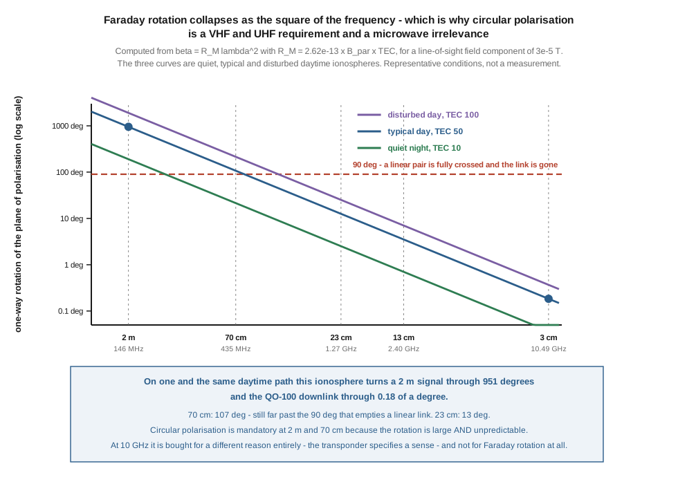
The first is that the case for circular polarization is a frequency-squared argument, and it collapses. §3 computes the ionospheric Faraday rotation from its own formula across six bands. On one daytime path the same ionosphere turns a 2 m signal through 951 degrees and the QO-100 downlink at 10.49 GHz through 0.18 of a degree. Circular polarization is mandatory at 2 m and 70 cm for exactly the reason usually given. At 10 GHz it is bought for a completely different reason, which the seed chapter never separates out.

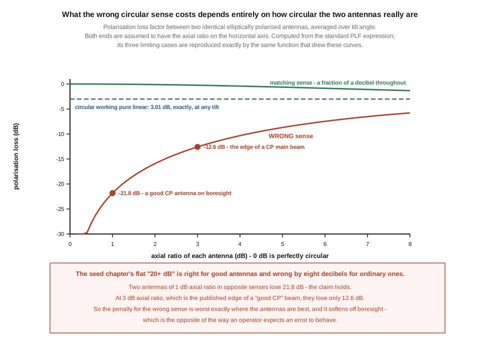
The second is that “the wrong sense costs 20+ dB” is true for good antennas and wrong by eight decibels for ordinary ones. §5 computes the polarization loss factor. Two antennas of 1 dB axial ratio in opposite senses lose 21.8 dB — the claim holds exactly. At the 3 dB axial ratio that marks the published edge of a “good CP” beam, they lose 12.6 dB. The penalty is worst where the antennas are best, and it softens as they degrade, which is the opposite of how an operator expects an error to behave.

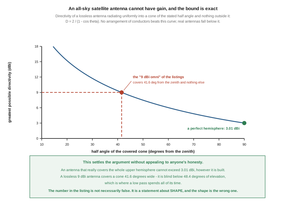
The third settles an argument this hobby has by assertion. The seed chapter dismisses the “9 dBi omnidirectional satellite antenna” as fiction. §7 shows it need not be fiction at all: a lossless antenna covering a cone and nothing outside it has a directivity of exactly 2 / (1 − cos θ), which puts a perfect upper hemisphere at 3.01 dBi and puts 9 dBi at a cone 41.6 degrees wide — blind below 48.4 degrees of elevation. The listing is a claim about shape, and the shape is the wrong one. Calling a real number a lie is the weaker argument and the more fragile one.

1.2 Three assumptions, all of them broken

The satellite problem is not one problem. It is three, they are independent, and nearly every design decision in this dive is traceable to one of them.

The target moves, and it moves in two axes. A low-earth-orbit satellite at 400 to 800 km has an orbital period between about 92 and 101 minutes, and from any one ground station a usable pass lasts roughly five to fifteen minutes from acquisition to loss of signal. During that window azimuth and elevation both change continuously, and the rate is set by the geometry of the particular pass rather than by anything the operator controls. This is what forces the whole question of whether to track at all, and if so with what. Vol 5 computes the slew rates involved and finds the answer is sharper than the folklore: on a 550 km orbit the azimuth rate at closest approach exceeds what a Yaesu G-5500DC can deliver only above 84.2 degrees of maximum elevation, and only about 2.6 % of passes climb that high.

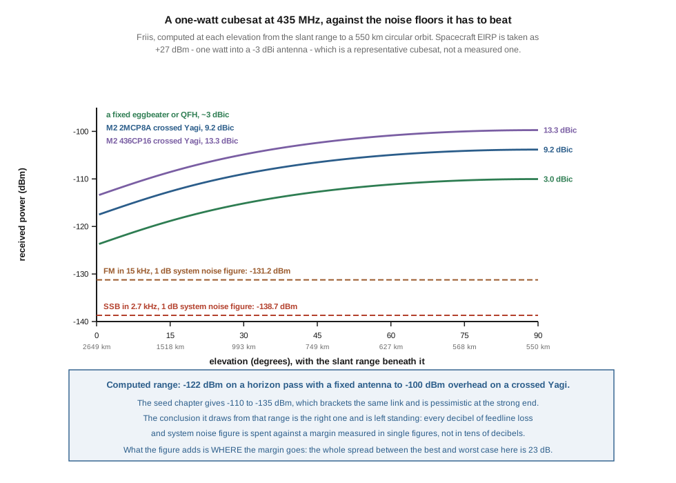
The link is power-starved. A cubesat transmits a fraction of a watt through an antenna with no gain to speak of, across hundreds or thousands of kilometres of slant range. §8 works the budget. The answer lands between roughly −100 and −122 dBm depending on the pass and the antenna, against a noise floor in the −131 to −139 dBm region: a margin measured in single figures and low tens of decibels, never in the comfortable tens that terrestrial VHF work enjoys. That is why the low-noise amplifier goes at the antenna rather than at the radio, why the coax run is kept short, and why at 10 GHz there is no coax run at all. Vol 4 quantifies each of those.

The polarization wanders, for two unrelated reasons. The ionosphere rotates the plane of a linearly polarized wave by an unpredictable and time-varying amount, and the spacecraft itself rotates its own antenna relative to the ground station. §3 and §4 take these separately because they scale differently, and conflating them is one of the ways the usual account goes wrong.

The three constraints do not weight equally across the spectrum, and that is the organising idea of this dive. At 2 m and 70 cm all three bite. At 23 cm the polarization problem has largely gone and the link-budget problem has got worse. At 10 GHz on a geostationary bird the pointing problem has vanished entirely — the antenna is aimed once and bolted down — the polarization problem is negligible, and the entire difficulty is the link budget and the stability of a local oscillator. The hardware looks completely different at each end of that range because the problem is a different problem.

1.3 Faraday rotation, computed rather than asserted

A linearly polarized wave crossing a magnetised plasma has its plane of polarization rotated. The rotation is

beta = R_M · lambda²

with the rotation measure given in SI units by

R_M ≈ 2.62 × 10⁻¹³ T⁻¹ · ∫ n_e(s) · B_∥(s) ds

where n_e is the electron density along the path and B_∥ the component of the geomagnetic field along the line of sight. For a satellite path the integral of electron density is the total electron content, conventionally quoted in TEC units of 10¹⁶ electrons per square metre; daytime values run from a few TECU to around 100.

Two features of that expression do all the work. The first is the lambda²: rotation falls as the square of frequency, so a factor of ten in frequency is a factor of a hundred in rotation. The second is that everything else in it — electron content, the field component along a path that is itself sweeping across the sky — is varying on timescales of minutes and is not knowable in advance at a ground station.

The lead figure evaluates that expression for a line-of-sight field component of 3 × 10⁻⁵ T, which is representative of a mid-latitude path and is stated as an assumption rather than a measurement. The numbers are these:

Table 1 — The lead figure evaluates that expression for a line-of-sight field component of 3 × 10⁻⁵ T, which is representative of a mid-latitude path and is stated as an assumption rather than a measurement. The numbers are these

ionosphere	2 m (146 MHz)	70 cm (435 MHz)	23 cm (1.27 GHz)	L-band (1.69 GHz)	13 cm (2.40 GHz)	3 cm (10.49 GHz)
quiet night, TEC 10	190°	21.4°	2.5°	1.4°	0.7°	0.04°
typical day, TEC 50	951°	107°	12.6°	7.0°	3.5°	0.18°
disturbed day, TEC 100	1901°	214°	25.1°	14.1°	7.0°	0.37°

The threshold that matters is 90 degrees, because at 90 degrees of rotation a linearly polarized transmitting antenna and a linearly polarized receiving antenna are exactly crossed and the link is gone. On the typical daytime row, 2 m is past that threshold by a factor of ten and 70 cm by a factor of nearly four. Even on the quiet-night row, 2 m clears it twice over. This is not a marginal effect at VHF and UHF; it is a signal that appears and disappears several times in a pass, and the rate at which it does so is set by how fast the ionosphere and the path geometry are changing, not by anything at either end of the link.

At 23 cm the picture has already changed: 12.6 degrees of rotation costs a linear pair 20·log₁₀(cos 12.6°) = 0.11 dB, which is nothing. And at the QO-100 downlink frequency the rotation is under a fifth of a degree even on a disturbed day.

⭐ That last row is the one the seed chapter does not draw the conclusion from. Its account of circular polarization opens with Faraday rotation and then applies the conclusion uniformly to every antenna in the chapter, dish and LNB included. But QO-100’s transponder specifies circular polarization for reasons of its own — frequency reuse and a defined sense on a geostationary bird with a fixed attitude — and Faraday rotation has nothing to do with it. Building a 10 GHz feed circular because the ionosphere demands it is doing the right thing for a reason that is false at that frequency, and an operator who believes the false reason will make the wrong call the first time a trade-off appears. Vol 4 states the actual reason.

⚠ One caveat belongs with the table, and it is a real limitation rather than a hedge. The rotation measure is computed here from a single representative field component and a uniform electron content; a real path integrates a field that varies along it and an ionosphere that is structured. The numbers are correct to their stated inputs and are the right order of magnitude; they are not a prediction for any particular pass. The conclusion they support — that the rotation is large, frequency-squared, and unpredictable at VHF and UHF — does not depend on the precision.

1.4 The second rotation, which has nothing to do with the ionosphere

Faraday rotation is a property of the medium. Spin fading is a property of the spacecraft, and the two are usually run together in a single paragraph that obscures the fact that they behave differently.

A great many amateur satellites and nearly every cubesat are not three-axis stabilised. Some are passively magnetically stabilised, some are spin-stabilised deliberately, and some are simply tumbling. Whichever it is, the spacecraft antenna’s orientation relative to the ground station changes on a timescale of seconds to tens of seconds. For a linearly polarized spacecraft antenna working a linearly polarized ground antenna, that alone produces the same deep periodic fading as Faraday rotation does.

The distinction is worth keeping because the two scale differently. Faraday rotation is a strong function of frequency — the whole content of §3. Spin fading is not a function of frequency at all. A tumbling spacecraft with a linear antenna produces the same polarization mismatch at 10 GHz as at 146 MHz, because the mechanism is mechanical. So the argument that the polarization problem goes away at microwave frequencies is only half true: the ionospheric half goes away, and the mechanical half does not.

For the hardware this matters at 23 cm and above, where §3’s table says Faraday rotation has become negligible but where a tumbling amateur payload has not become any more stable. It is why circular polarization is still worth having on a 23 cm cubesat downlink even though the ionosphere no longer requires it, and it is a distinct claim from the one the ionosphere supports.

There is a third mechanism that gets folded into “polarization problems” and should not be. At low elevation a signal arrives both directly and by a ground reflection, and the reflection is delayed and has its polarization altered. The resulting interference produces deep nulls that look like polarization fading and are not: they are multipath, they depend on antenna height above the reflecting surface, and circular polarization does not fix them. It does something narrower and genuinely useful, which is that a single specular reflection reverses the sense of a circularly polarized wave, so a correctly-sensed CP antenna rejects the once-reflected ray by the figure §5 computes rather than adding it to the direct ray with an arbitrary phase. That is a real benefit and it is not the same benefit as immunity to Faraday rotation.

1.5 What circular polarization costs, and what the wrong sense costs

A circularly polarized wave is two orthogonal linear components of equal amplitude in time quadrature. Following the IEEE convention — looking along the direction of propagation, from behind the receding wave — a clockwise-rotating field vector is right-hand circular (RHCP) and a counter-clockwise one is LHCP. Optics uses the opposite convention, which is a standing source of confusion and is why every serious specification states which convention it means.

No real antenna produces perfect circularity. The quality of the circularity is the axial ratio: the ratio of the major to the minor axis of the polarization ellipse actually radiated, conventionally in decibels, AR(dB) = 20·log₁₀(E_max / E_min). Zero decibels is a perfect circle; infinity is pure linear.

The coupling between any two elliptically polarized antennas follows from their two axial ratios, their senses, and the difference in the tilt angles of their ellipses:

PLF = ½ + [ s·4·r₁·r₂ + (r₁² − 1)(r₂² − 1)·cos 2Δ ] / [ 2·(r₁² + 1)(r₂² + 1) ]

with r the axial ratio as a voltage ratio, s = +1 for matching senses and −1 for opposite, and Δ the tilt difference. A tumbling spacecraft sweeps Δ through everything, so the tilt-averaged case (cos 2Δ = 0) is the right statistic for a satellite link, and it is what the figure plots.

Three limiting cases fall out of that expression, and the function that drew the figure reproduces all three exactly, which is the check that it was entered correctly:

• Two perfect circular antennas of the same sense: 0.0000 dB. No loss, at any tilt.
• A perfect circular antenna working a purely linear one: exactly 3.0103 dB, whatever the linear antenna’s tilt angle. This is the famous 3 dB, and it is not an approximation — it is 10·log₁₀(½), arising because a linear antenna can only couple to one of the two quadrature components.
• Two perfect circular antennas of opposite sense: a complete null.

That third case is where the usual account goes wrong, because no real antenna is perfect and the null is extraordinarily sensitive to how imperfect it is. Evaluating the same expression at realistic axial ratios:

Table 2 — That third case is where the usual account goes wrong, because no real antenna is perfect and the null is extraordinarily sensitive to how imperfect it is. Evaluating the same expression at realistic axial ratios

axial ratio at both ends	matching sense	wrong sense
0 dB (ideal)	0.00 dB	complete null
1 dB	0.03 dB	21.8 dB
2 dB	0.11 dB	15.9 dB
3 dB	0.25 dB	12.6 dB
6 dB	0.90 dB	7.0 dB

🔴 The seed chapter’s “20+ dB” is correct as a headline and misleading as a rule. It holds at 1 dB axial ratio, which is what a well-made helix or a good crossed Yagi achieves on boresight. It does not hold at 3 dB, which is the axial ratio that conventionally defines the edge of a usable CP beam — and there the penalty is 12.6 dB. The number the seed quotes and the number an operator will actually meet differ by nine decibels.

⭐ The direction of the error is the interesting part. The rejection is deepest where the antennas are cleanest and shallows as they degrade. So the wrong sense is at its most catastrophic on boresight, in the middle of a good pass, with a well-built antenna — and it partially forgives itself at the edges of the beam, at low elevation, and on a cheap antenna. An operator diagnosing a “mysteriously deaf” station will find the symptom strongest exactly where the equipment is working best. That is a diagnostically awkward signature and it is worth knowing before chasing it.

⚠ And the matching-sense column deserves a note, because it is the case for CP stated properly. A matching-sense CP pair loses a quarter of a decibel at 3 dB axial ratio and 0.9 dB at 6 dB. Against that, a linear-to-linear path suffers the §3 rotation: anything from zero to a complete null, unpredictably, several times a pass. The trade is not “3 dB for convenience”. It is a fixed fraction of a decibel, or a fixed 3.01 dB against a linear counterpart, in exchange for removing a 0-to-infinity variable. Stated that way the case for circular polarization is stronger than the usual framing makes it, not weaker.

1.6 Axial ratio is a property of a direction, not of an antenna

A specification sheet quotes one axial ratio. An antenna has a different one in every direction, and the number quoted is the best one it ever achieves, on boresight, at the design frequency.

This is not a minor caveat. It restructures what a “CP antenna” means. The region over which an antenna holds a usable axial ratio — the CP beamwidth — is narrower than its half-power beamwidth, often considerably. An antenna that is 1 dB axial ratio on axis may be 6 dB at 45 degrees off axis, at which point §5’s table says it is 0.90 dB down against a matching-sense partner and, more importantly, only 7.0 dB up on the wrong sense. Over part of its pattern a CP antenna is, in polarization terms, barely circular.

Three practical consequences follow, and they point in different directions for different antennas.

For a fixed all-sky antenna — a turnstile, an eggbeater, a quadrifilar helix — the axial ratio is at its best near the zenith and degrades toward the horizon, which is precisely backwards from where the help is needed. A bird at 10 degrees elevation is at its longest slant range, in the worst multipath, at the edge of the pattern and being received with the worst polarization the antenna offers. Vol 2 is about the antennas that trade absolute gain for a pattern shape that limits how bad that gets.

For a tracked gain antenna the consequence is the reverse and is more forgiving: if the bird is centred in the main beam it is also in the best-polarized part of the pattern, so pointing accuracy buys polarization quality as well as gain. Vol 3 covers those, and notes that the axial-mode helix in particular holds a good axial ratio across an unusually wide beam, which is why it tolerates a rough rotator.

For specification reading, the rule is that a CP antenna quoted without an axial ratio figure has told the reader nothing about its polarization, and one quoted without the angle at which the axial ratio applies has told the reader only its best case. Vol 5’s commercial survey applies that test and finds it disqualifies a good deal of what is sold.

1.7 The gain bound on all-sky coverage

The seed chapter’s myth list contains this: “‘9 dBi omni’ is a physical impossibility… a high gain figure on an ‘omnidirectional satellite antenna’ listing means either the pattern is not actually omni or the dBi number is fiction.”

The second half of that sentence is right and the first half is wrong, and the distinction is worth making carefully, because declaring a real thing fictitious is a failure mode this program has committed before.

Directivity is the ratio of the power density radiated in the best direction to the average over all directions. For a lossless antenna that radiates uniformly into a cone of half angle θ and nothing outside it — the most generous possible idealisation of an antenna with a defined coverage region — the solid angle of the cone is 2π(1 − cos θ) steradians out of 4π, so

D = 4π / [2π(1 − cos θ)] = 2 / (1 − cos θ)

This is a hard upper bound. No arrangement of conductors beats it, because it assumes a perfectly uniform pattern inside the coverage region and an absolute null outside it, which nothing achieves. Real antennas fall below the curve.

Evaluating it:

Table 3 — Evaluating it

coverage	half angle	greatest possible gain
the whole upper hemisphere	90°	3.01 dBi
down to 30° elevation	60°	6.02 dBi
down to 48.4° elevation	41.6°	9.00 dBi
down to 60° elevation	30°	11.7 dBi

⭐ So 9 dBi is perfectly achievable, and an antenna that has it is blind below 48.4 degrees of elevation. That is not a defect in the specification; it is what 9 dBi means. The listing is making a true statement about gain and an implicit false statement about coverage, and the honest correction is to that second half rather than to the number.

The consequence for satellite work is decisive, and it is why Vol 2 exists as a separate volume from Vol 3. On a 550 km orbit, about 39 % of passes reach above 30 degrees elevation and only 6.7 % reach above 75 degrees (Vol 5 computes these). A fixed antenna concentrating its pattern into the top 41.6 degrees of the sky misses the great majority of every pass, including all of acquisition and all of loss of signal — the parts where a beacon is first heard and last heard.

An antenna intended to work the whole sky without being pointed therefore wants low gain, deliberately, and what it wants in exchange is a flat pattern and a good axial ratio at low elevations. The 3.01 dBi hemispherical bound is the budget such an antenna is spending, and a real one — a quadrifilar helix, an eggbeater — comes out a little above it over part of the dome and below it elsewhere, because the real pattern is not a top hat.

Two further points that follow from the same arithmetic. First, an antenna that is omnidirectional in azimuth is not bound by this curve at all: a collinear can have 9 dBi honestly by squashing its pattern into a thin disc at the horizon, which is a perfectly good terrestrial antenna and a perfectly useless satellite one. The bound applies to hemispherical coverage, not to azimuthal omnidirectionality, and the two are routinely confused in exactly these listings. Second, adding a reflecting screen below a turnstile buys up to 3 dB by halving the covered solid angle — the same arithmetic read forwards — which is why Vol 2’s fixed antennas nearly all have one.

1.8 The link budget, and where the margin actually goes

The seed chapter states that a satellite downlink lands “somewhere in the −110 to −135 dBm range”. That is a reasonable bracket asserted without a calculation, and since every argument about preamps and feedline in Vol 4 rests on it, it is worth doing the calculation.

Take a representative amateur cubesat: one watt into an antenna with −3 dBi in the direction of the ground station, so an EIRP of +27 dBm. Take a 550 km circular orbit, which gives a slant range of 550 km overhead and 2,649 km at the horizon. Friis gives the free-space path loss at 435 MHz, and three ground antennas span the realistic range — a fixed all-sky antenna at about 3 dBic, and the two M2 crossed Yagis whose published gains are 9.2 and 13.3 dBic.

Table 4 — 8. The link budget, and where the margin actually goes

ground antenna	5° elevation	30° elevation	overhead
fixed all-sky, ~3 dBic	−122.1 dBm	−118.7 dBm	−110.0 dBm
crossed Yagi, 9.2 dBic	−115.9 dBm	−112.5 dBm	−103.8 dBm
crossed Yagi, 13.3 dBic	−111.8 dBm	−108.4 dBm	−99.7 dBm

Against those, the thermal noise floor in the receiver bandwidth with a 1 dB system noise figure is −138.7 dBm for a 2.7 kHz SSB channel and −131.2 dBm for a 15 kHz FM channel.

⚠ The seed’s bracket is confirmed in substance and is pessimistic at the strong end, and the correction is small enough that the honest treatment is to say so rather than to make a meal of it. The computed range runs from −122 dBm to −100 dBm across the cases that matter; −135 dBm belongs to a weaker spacecraft or a higher orbit than the one specified. The conclusion the seed draws from the bracket is right and is left standing.

What the calculation adds is the structure inside the range, and that is where the engineering is.

The spread from the worst realistic case to the best is 22.4 dB, and it decomposes cleanly: 12.1 dB of it is the slant range between horizon and zenith, and 10.3 dB is the choice of ground antenna. Those are the same order of magnitude, which is the first useful thing the table says — choosing a tracked gain antenna over a fixed one buys about as much as the difference between the worst and best moment of a pass.

The FM case has margin and the SSB case has less than it looks. A fixed antenna on an FM bird at 5 degrees sits 9.1 dB above the noise floor, which is thin but workable, and 21.2 dB above it overhead. The SSB case is nominally more comfortable because the narrower channel lowers the floor by 7.5 dB — but SSB on a linear transponder is being demodulated by ear against a continuously moving Doppler offset, so the usable threshold sits well above the noise floor rather than at it.

And every one of those numbers assumes a 1 dB system noise figure, which is only obtainable with a low-noise amplifier at the antenna. Vol 4 computes what happens otherwise: with 3 dB of coax between antenna and shack, the same station runs at a 3.61 dB system noise figure with the preamp at the radio and 9.00 dB with no preamp at all. Reading those against this table: the no-preamp station has lost 8 dB, which is most of the difference between a fixed antenna and a 13.3 dBic crossed Yagi. The cheapest decibels in a satellite station are not in the antenna.

1.9 Where this dive stops and the tracking dive starts

The satellite material in this project is split across two dives, and the split is not arbitrary. It is worth stating precisely, because the seed chapter’s own cross-references to the companion are wrong and because the reader needs to know which document answers which question.

This dive owns the hardware in the signal path and the machinery that moves it. The radiating element and its polarization (Vol 2 and Vol 3), the dish, the feed, the LNB and the chain of active parts behind them (Vol 4), and the az/el rotator considered as a mechanism — its gear train, its position feedback, the torque and wind load it must survive, and how to size and buy one (Vol 5).

The companion dive at /satellite-tracking/ owns the prediction and the control. Orbital mechanics and the Keplerian elements, the two-line element format, SGP4 propagation, the transformation that turns an orbit into a look angle for a particular ground station, the Doppler derivation, the tracking programs, and the controller protocols and software that turn a predicted look angle into a slew command.

The boundary is the slew command. Where the azimuth and elevation numbers come from is the tracking dive’s subject. What happens mechanically when the rotator receives them is this dive’s. Where the two meet — the rotator’s electrical interface and its position feedback — is described here as a property of the hardware and driven there as a control problem.

The same rule settles the two topics that genuinely straddle the line.

The zenith keyhole is a geometric fact with a hardware consequence and a software mitigation. Vol 5 computes the azimuth rate a pass demands and compares it with what real rotators deliver, because that is a specification an operator buys against. The mitigations — flipping the elevation axis past 90 degrees so azimuth can stay put, or leading and lagging azimuth through the turn — are behaviours of tracking software and belong there.

Doppler is not a hardware question at all. It is a tuning problem, and the derivation, the sign conventions for V/U against U/V birds, and the closed-loop correction all belong to the companion dive. It appears in this dive exactly twice: once in Vol 4, where the local-oscillator stability of a 10 GHz LNB is compared against a channel width, which is a hardware specification; and once here, to say that it is out of scope.

⚠ A note on how the companion is referenced, because it is a correction to the seed. The seed chapter cross-references the tracking dive as “Vol 34” in nine places. In the hub’s volume map, Vol 34 is this volume and the tracking dive is Vol 35 — so every one of those references points at the document making them. One of the seed’s own figures has it right and says “Vol 35”, which is the giveaway that the numbering drifted rather than that anyone chose it. This dive avoids the whole class of error by referencing the companion only by its landing URL, /satellite-tracking/, and never by a volume number: that dive has not yet been expanded, and its internal numbering will change when it is.

1.10 Resources

• Kraus, Antennas — the axial-mode helix, its gain expression and the conditions for axial-mode operation. Vol 3 works through that expression and the extent to which it overstates real gain.
• Balanis, Antenna Theory: Analysis and Design — the polarization-loss factor of §5 in its general form, and the definition of axial ratio used throughout this dive.
• The Faraday-rotation expression of §3, beta = R_M lambda² with R_M ≈ 2.62 × 10⁻¹³ T⁻¹ ∫ n_e B_∥ ds, is the standard SI form. The TEC values are representative daytime and night-time figures; no measured ionospheric profile was used and none is claimed.
• AMSAT (amsat.org) — the satellite status board, frequency lists and ground-station notes. The list of currently-active birds in Vol 2 and Vol 3 was read from it on 17 September 2026.
• AMSAT-DL (amsat-dl.org) — the QO-100 narrowband and wideband transponder band plans used in Vol 4.
• Satellite tracking — the companion dive: orbital mechanics, TLEs, SGP4, look angles, Doppler, and the three paths to driving a rotator. §9 states the boundary.
• Antenna theory and practice — polarization, gain, directivity and the Friis equation, if any of §5’s or §7’s vocabulary needs shoring up.
• Transmission lines and feedlines — loss per unit length against frequency, which is the quantity Vol 4’s feedline argument turns on.
• Yagi-Uda antennas — the parasitic-array theory that Vol 3’s crossed Yagis assume rather than re-derive.
• Active splitters, distribution amplifiers and preamps — masthead LNAs and bias-tee arrangements, of which Vol 4 covers only the satellite-specific parts.