Pointing At It: Crossed Yagis, Handheld Beams and the Axial-Mode Helix

---

3.1 About this volume

Vol 2 covered the antennas that cover the whole sky and are never pointed. This one covers the antennas that are pointed, and the machinery that points them is Vol 5.

The organising fact is Vol 1 §7’s bound: a fixed all-sky antenna has at most 3.01 dBi to spend, so the entire case for a rotator, a controller, a cross-boom and a control cable is the 6 to 10 dB that a tracked array has and a fixed one cannot. §2 asks what that buys against Vol 1 §8’s link budget, and the answer is narrower than the hobby’s enthusiasm for rotators suggests.

Three results in this volume differ from the seed chapter.

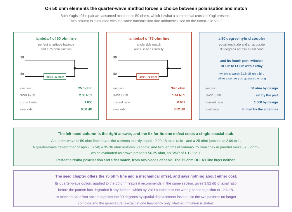
The quarter-wave phasing method has a cost the seed does not mention, and on the antennas it recommends in the same section the cost is severe. §3 evaluates all three phasing methods as drawn. On two Yagis matched to 50 Ω — which is what a commercial crossed Yagi presents — a quarter-wave of 75 Ω line leaves the two currents in a ratio of 0.667, an axial ratio of 3.52 dB, on boresight, before the pattern has degraded it any further. A quarter-wave of 50 Ω line instead gives perfect amplitude balance and a 25 Ω junction, and a second quarter-wave stub restores 50 Ω. Perfect circular polarization is available from two pieces of cable, and the seed recommends the option that is not.

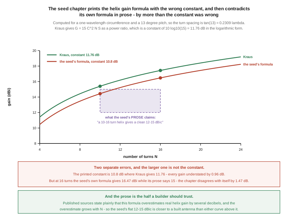
The helix gain formula is printed with the wrong constant, and then contradicted by the chapter’s own prose by more than the constant is wrong. §7 works it. Kraus’s expression carries a constant of 10·log₁₀(15) = 11.76 dB; the seed prints 10.8, understating every helix by 0.96 dB. But the seed’s prose then claims that “a 10–16 turn helix gives a clean 12–15 dBic”, where its own formula at 16 turns gives 16.47 dBi — a self-contradiction of 1.47 dB on top of the constant. ⚠ And the prose is the half a builder should trust, for a reason §7 sets out.

The axial-mode helix’s real advantage is not gain. It is that the geometry produces the quadrature, so there is no phasing network, and therefore nothing that can be built backwards. Every defect in §3 is a defect a helix cannot have. §8 quantifies what it gives instead: 0.42 dB of axial ratio at ten turns, over a 34-degree beam.

3.2 What tracking actually buys

The published gain of the two crossed Yagis in M2’s LEO Pack is 9.2 dBic on 2 m and 13.3 dBic on 70 cm. Against Vol 2’s fixed antennas at about 3 dBic, that is 6.2 and 10.3 dB.

Read against Vol 1 §8’s budget, which computed the same link across a pass at 550 km, those decibels have a specific and slightly deflating interpretation. The range term alone varies by 12.1 dB between a horizon pass and an overhead one. So the 70 cm crossed Yagi buys somewhat less than the difference between the best and worst moment of a single pass, and the 2 m one buys about half of it.

That is not an argument against tracking; it is an argument for knowing what the purchase is. There are three cases where it is decisive and they are worth naming, because outside them a fixed antenna is the better engineering.

A link with a hard threshold. An FM bird degrades gracefully: 6 dB of extra gain turns a noisy contact into a clean one. A digital downlink does not — below its demodulation threshold there is nothing at all. Vol 2 §8 noted that this is exactly what the loss of APT did to 137 MHz weather work, and the same logic governs L-band and the QO-100 wideband transponder in Vol 4. Where the threshold is hard, gain converts directly into whether the station works.

A weak linear transponder worked on SSB. Vol 1 §8 put a fixed antenna at −118.7 dBm at 30 degrees elevation against a −138.7 dBm noise floor in an SSB channel. Twenty decibels sounds ample and is not, because SSB on a linear bird is demodulated by ear against a continuously moving Doppler offset and the usable threshold sits well above the noise floor. The crossed Yagi’s 10 dB is the difference between straining and working.

An uplink. Everything above concerns receiving. On transmit the gain figure is EIRP, and there is no substitute for it short of a bigger amplifier — which is the more expensive decibel, and the one that makes the station a nuisance if it is overdone.

⭐ And there is a fourth consideration that runs the other way and is usually left out. Vol 5 computes that on a 550 km orbit the azimuth rate at closest approach exceeds what a Yaesu G-5500DC delivers above 84.2 degrees of maximum elevation. Those passes — the highest, shortest-range, strongest ones — are precisely where a tracked array fails and a fixed antenna does not. The tracked station’s advantage is smallest on the best passes. It is not a large effect, because only about 2.6 % of passes climb that high, but it is the opposite of what an operator buying a rotator expects.

3.3 Crossed Yagis, and the ninety degrees

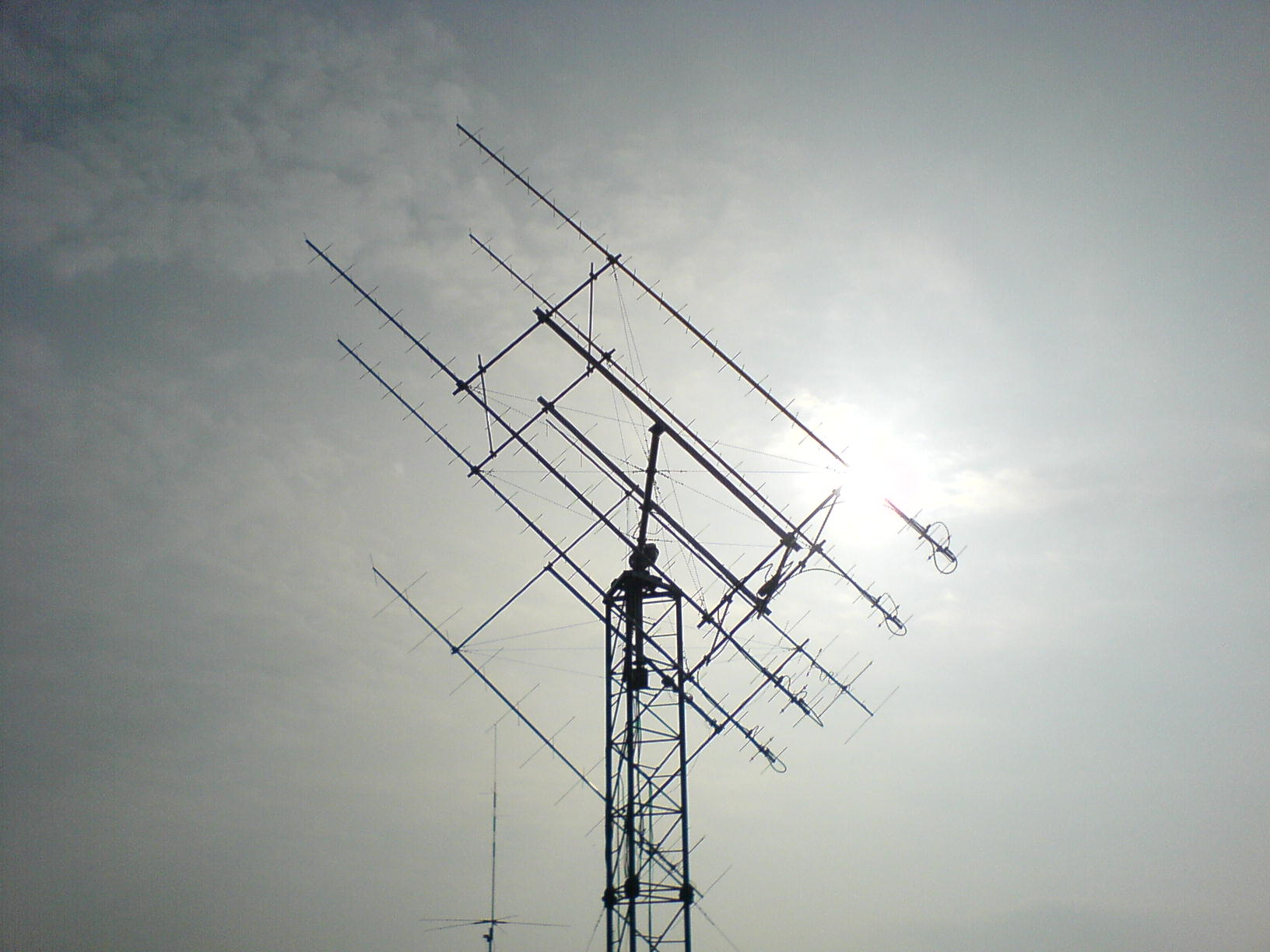
The workhorse tracked satellite antenna is a pair of Yagis on a common boom, rotated 90 degrees from one another and fed in phase quadrature. The Yagi theory — parasitic coupling, boom length against gain, the matching topologies — is the Yagi-Uda dive’s subject and is assumed here. The new element is the crossing and the phasing, and that is where the errors live.

One structural point first, carried over from Vol 2 §3 and equally load-bearing here: two perpendicular co-located driven elements have zero mutual impedance, so each Yagi presents its own feedpoint impedance regardless of the other. A crossed pair can therefore be designed as two independent antennas that happen to share a boom, which is why the arithmetic below is as simple as it is.

3.3.1 The three methods, evaluated as drawn

The lead figure evaluates each, assuming both Yagis are matched to 50 Ω — which is what a commercial crossed Yagi presents and what a builder following a published design will have.

Table 1 — The three methods, evaluated as drawn

method	junction	SWR to 50 Ω	current ratio	axial ratio
λ/4 of 50 Ω line	25.0 Ω	2.00:1	1.000	0.00 dB
λ/4 of 75 Ω line	34.6 Ω	1.44:1	0.667	3.52 dB
90° quadrature hybrid	50 Ω by design	set by the part	1.000 by design	limited by the antennas

The arithmetic is Vol 2 §3’s, unchanged: the delayed branch presents Z₀²/Z_d at the junction in parallel with the direct one, and the current ratio between the two antennas is Z_d/Z₀.

🔴 The seed chapter offers the quarter-wave line and the mechanical offset, and states the cost of neither. Its quarter-wave option, applied to the 50 Ω Yagis it recommends in the same section, gives 3.52 dB of axial ratio on boresight. Reading that against Vol 1 §5’s table: at 3.52 dB axial ratio the rejection of the wrong circular sense has fallen from the 21.8 dB the chapter claims elsewhere to about 12 dB, and the antenna has become noticeably elliptical before its pattern has degraded it at all. This is not a small effect and it is entirely avoidable.

⭐ The fix is one extra piece of cable, and it is the result worth taking from this section. Use a quarter-wave of 50 Ω line for the delay. The currents then come out exactly equal — Z_d/Z₀ = 1 — so the axial ratio is limited only by the antennas themselves, and the junction sits at 25 Ω, a 2:1 match. A quarter-wave transformer of √(25 × 50) = 35.36 Ω restores 50 Ω. Coax of 35 Ω is not a stock item, but two equal lengths of ordinary 75 Ω cable in parallel make 37.5 Ω, and evaluating that as drawn gives 37.5²/25 = 56.25 Ω, an SWR of 1.125:1. Two pieces of RG-59 buy perfect amplitude balance and a flatter match than the 75 Ω shortcut delivers.

⚠ The mechanical-offset method has its own unstated costs. Both Yagis are fed in phase and one is slid a quarter-wavelength forward along the boom, letting the spatial displacement supply the quadrature. This avoids the phasing line entirely, which is its attraction. But the two patterns are then no longer coincident — the array’s phase centres are a quarter-wave apart — and the displacement is exactly a quarter-wave at one frequency only, so the axial ratio degrades away from the design frequency in a way the line method does not. The seed mentions neither limitation.

The hybrid coupler is the correct answer for a station that can afford it, and its advantages are not only in this table. It gives equal amplitude and an accurate 90 degrees across a real bandwidth rather than at a point, it presents a designed 50 Ω, and its fourth port makes the sense switchable. §4 is about that last property.

⚠ The seed names a specific coupler and this dive does not repeat it. Its figure annotates the hybrid as “e.g. an SP-70 / ARR coupler”. No product matching either designation could be verified on 17 September 2026: Advanced Receiver Research’s site presents product categories whose listings could not be retrieved, and no “SP-70” coupler could be matched to any manufacturer. The device class is entirely real and widely used — that is not in question — but the model designation is withdrawn rather than repeated, on this program’s standing rule that an unverifiable product row is dropped and not replaced with a guess.

3.4 Switchable sense, and what it is worth

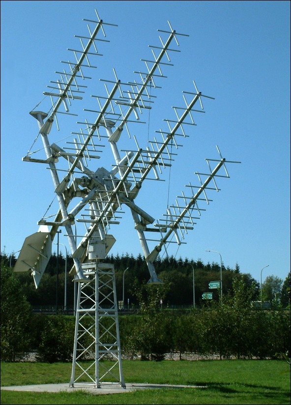
Vol 1 §5 computed that two antennas of 1 dB axial ratio in opposite circular senses lose 21.8 dB, and that the penalty falls to 12.6 dB when both are at 3 dB axial ratio. That number is what a switchable-sense feed is buying, and it is worth stating what the purchase actually is, because it is easy to misdescribe in both directions.

It is not insurance against building the antenna wrong. A relay that swaps RHCP for LHCP does exactly that and nothing more; it does not compensate an axial ratio, fix a phasing error, or help with Faraday rotation. If the array is built with a 3.5 dB axial ratio because of §3’s 75 Ω shortcut, switching the sense leaves it at 3.5 dB.

It is a way of choosing per bird, and of discovering which sense a bird actually uses. Amateur satellites vary: most that specify a sense use RHCP, some use LHCP, and a good many cubesats are linear or simply do not say. A ground station with a fixed sense is at Vol 1 §5’s penalty on any bird that turns out to be the other one, and has no way to find out except by comparison with someone else’s station. A switchable one peaks whichever sense is stronger, which both recovers the loss and measures the bird.

And on a linear-polarized spacecraft the switch is worth nothing at all, which is the part most often left out. Vol 1 §5’s exact result is that a circular antenna working a purely linear signal loses 3.0103 dB whatever the tilt — and that is true of either sense equally. Against a linear cubesat, switching the relay changes nothing, and an operator who watches the signal not change has learned something useful about the spacecraft rather than about the relay.

The cost is the coupler, the relay, a control line up the mast, and the insertion loss of both — which at 70 cm, ahead of a masthead preamp, is spent directly against Vol 4’s noise-figure budget. For a station working one known bird it is not worth it. For a station working whatever is overhead it is one of the better decibels available.

3.5 Handheld beams — linear, and right to be

The simplest tracked station needs no rotator, no controller and no mast: a dual-band beam held in one hand, aimed by eye, walked across the sky. The two canonical antennas are the Arrow II 146/437 and the Elk 2M/440L5, and the seed chapter’s account of them is correct in substance and contains one editorial artefact worth flagging.

The Arrow II 146/437-10 carries 3 elements for 2 m and 7 elements for 70 cm on a 37½-inch boom, the two element sets mounted perpendicular to one another. ⚠ That perpendicularity is cross-band isolation, not circular polarization, and it is the single most common misreading of these antennas. Arrow’s own description says “3 Elements for 2 Meters crossed with 7 Elements for 70 cm” — the word “crossed” there means the 2 m elements are at right angles to the 70 cm elements so that the two bands interact as little as possible on a shared boom. There is no phasing network and no quadrature. The antenna is linearly polarized on both bands.

⭐ The seed chapter gets this right, and its text records the author working it out in real time. It reads: “the Arrow II 146/437 (a crossed… actually dual-band Yagi with separate 2 m and 70 cm element sets on one boom…)”. The ellipsis and the “actually” are an unedited self-correction left in published prose. The conclusion it arrives at is the right one and is confirmed here; only the editing is at fault, and it is recorded because a reader encountering “a crossed… actually” reasonably wonders which half to believe.

The Elk 2M/440L5 is a dual-band log-periodic rather than a Yagi — every element is driven, which is what gives it smooth coverage across both bands in a lighter package — and it is likewise linear.

3.5.1 Why linear is the right choice here, and not a compromise

Being linear costs these antennas Vol 1 §5’s exact 3.01 dB against any circularly polarized spacecraft. Three things pay for it.

The operator is the polarization control. A handheld beam is rotated about its own boom axis while it is being aimed, so the operator can peak through Faraday rotation and spin fading by wrist alone — a manual, closed-loop polarization tracker that a mast-mounted array cannot have. Vol 1 §3 computed 951 degrees of rotation at 2 m on a typical day, which sounds hopeless until one notices that its rate is slow enough to follow by hand.

Circular polarization on a handheld would cost weight and balance, which are the binding constraints on an antenna held at arm’s length for ten minutes while walking.

And the birds these antennas are used on are the forgiving ones. They are FM satellites with strong beacons, where Vol 1 §8’s budget shows a comfortable margin and 3 dB is affordable.

This is the recommended entry point to satellite operating, and the seed chapter is right to say so: a beam, a dual-band handheld, and a pass prediction from /satellite-tracking/.

⚠ A photograph of either antenna is owed. The seed carried one captioned as an Elk 2M/440L5 and sourced from a marketplace listing; it could not be confirmed to be an Elk and has been withdrawn rather than re-captioned. Neither antenna is represented on Wikimedia Commons. The provenance file records the search.

3.6 The axial-mode helix, which needs no phasing network at all

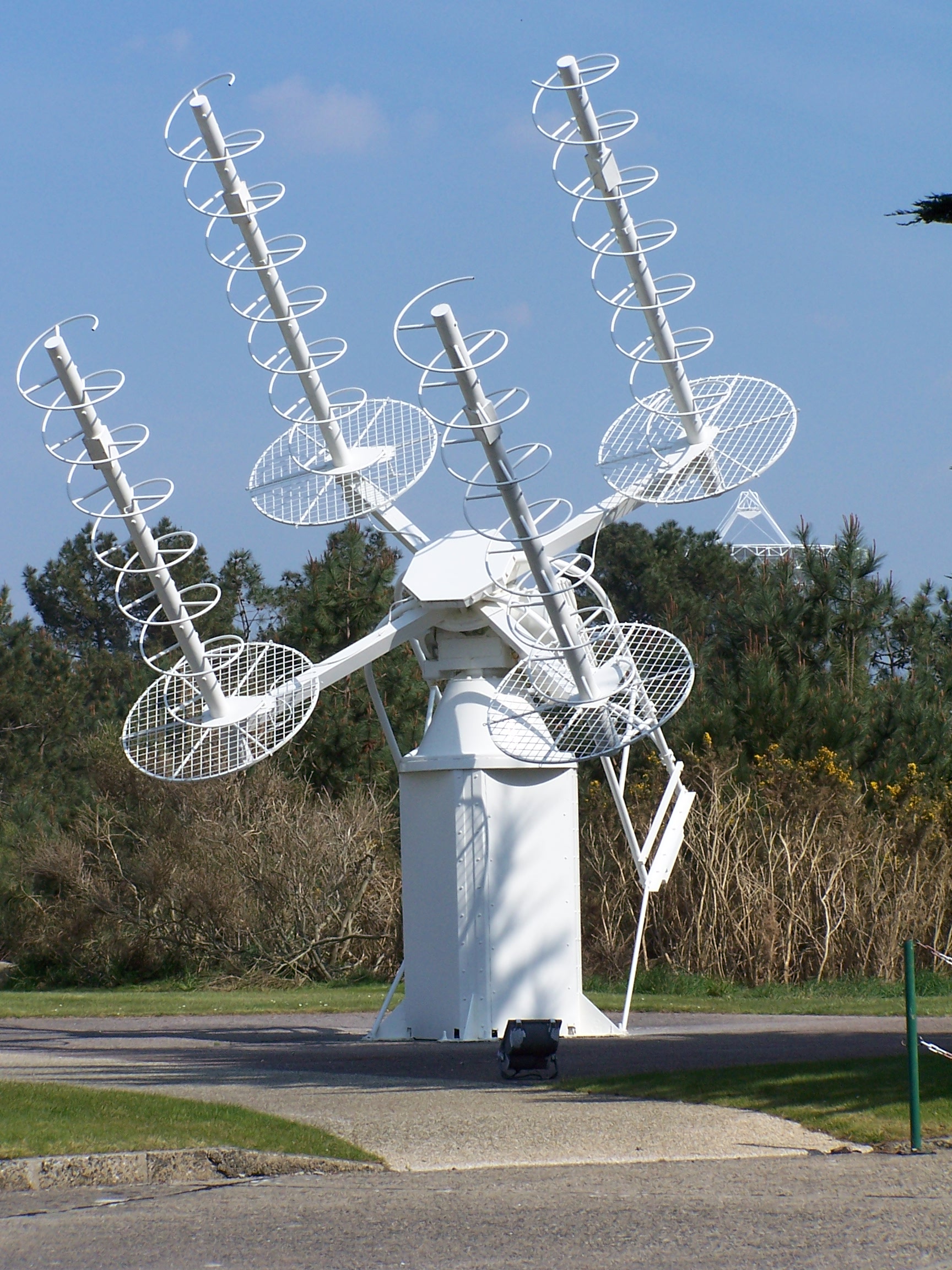
Everything §3 had to say about getting 90 degrees of phase into a pair of antennas simply does not arise for the axial-mode helix. Wind a conductor into a helix whose circumference is about one wavelength, over a ground plane, and it radiates an end-fire circularly polarized beam from a single feedpoint. The geometry produces the quadrature. There is no phasing line, no hybrid, no relay, and — the point that matters most given what §3 found — nothing that can be connected backwards.

The current travelling along the helical conductor is itself rotating in space at the rate the helix is wound, and when the circumference is near a wavelength the fields from successive turns add in the axial direction with the progressive phase that circular polarization requires. The sense follows the winding: a right-hand wound helix radiates RHCP.

That last property is the design’s one inflexibility, and the seed chapter states it correctly: the handedness cannot be changed without rewinding. A helix cannot be relay-switched the way §4’s hybrid-fed crossed pair can. It is built for one sense, and if the target bird turns out to use the other, Vol 1 §5’s penalty applies with nothing to be done about it short of a second antenna.

Against that, the helix has three properties that make it the right choice more often than its popularity suggests.

Its axial ratio is excellent and improves with length. §8 computes it: Kraus’s expression (2N+1)/2N gives 0.42 dB at ten turns and 0.27 dB at sixteen. Compare §3’s table, where the best a quarter-wave-fed crossed pair achieves is limited by the cable impedance chosen and the worst is 3.52 dB.

Its beam is broad for its gain, which means it tolerates pointing error. §8 gives 34 degrees of half-power beamwidth at ten turns. A rotator with a couple of degrees of backlash and a potentiometer that has drifted with temperature is of no consequence against a 34-degree beam, and Vol 5 notes that this is what makes the helix the natural partner for a budget or home-built rotator.

Its feedpoint is real and broad. Roughly 140 · C_λ ohms, so about 140 Ω for a one-wavelength circumference, resistive across a wide band. It needs a match to 50 Ω, but it does not need a tuner, and its bandwidth is set by the axial-mode window rather than by a resonance.

The helix is at its best at 70 cm and 23 cm as a standalone tracked antenna, and at 13 cm and above as a dish feed — which is Vol 4’s subject.

3.7 The gain expression, printed wrong and then contradicted

Kraus’s gain expression for an axial-mode helix is usually written as a power ratio:

G ≈ 15 · C_λ² · N · S_λ

with C_λ the circumference and S_λ the turn spacing, both in wavelengths, and N the number of turns. Put into decibels, that constant becomes 10·log₁₀(15) = **11.76 dB**, and the expression reads G(dBi) = 11.76 + 10·log₁₀(C_λ² N S_λ).

The seed chapter prints it as G ≈ 10.8 + 10·log₁₀(C²NS/λ³). The variable grouping is right — C²NS/λ³ is C_λ² N S_λ — and the constant is wrong by 0.96 dB, understating every helix in the chapter.

That is the smaller of the two errors.

At a 13-degree pitch the turn spacing is tan 13° = 0.2309 λ, so for a one-wavelength circumference:

Table 2 — At a 13-degree pitch the turn spacing is tan 13° = 0.2309 λ, so for a one-wavelength circumference

turns	Kraus, 11.76 dB constant	the seed’s formula, 10.8 dB	the seed’s prose
6	13.18 dBi	12.22 dBi	—
10	15.39 dBi	14.43 dBi	”12–15 dBic”
16	17.44 dBi	16.47 dBi	”12–15 dBic”
20	18.40 dBi	17.44 dBi	—

🔴 The chapter’s prose contradicts the chapter’s own formula, by more than the formula’s constant is wrong. It states that “a 10–16 turn helix gives a clean 12–15 dBic”. At sixteen turns its own equation returns 16.47 dBi — 1.47 dB above its own stated ceiling — and Kraus’s returns 17.44 dBi, 2.44 dB above it. A reader who trusts the formula and a reader who trusts the sentence will size the same antenna differently by up to two and a half decibels.

⭐ And the prose is the half a builder should trust, which is why this is a correction that has to be made carefully. Published sources state plainly that this formula overestimates real helix gain by several decibels, and that the overestimate grows with the number of turns — the expression is a small-N fit extrapolated past its range. So the seed’s flat “12–15 dBic” is, by accident, closer to what a built antenna will measure than either curve above it.

The honest correction is therefore not “the prose is wrong, use the formula”. It is:

• The constant is 11.76 dB, not 10.8. This is arithmetic and is not in dispute.
• The formula is an upper bound rather than a prediction, increasingly optimistic with N.
• A ten-turn helix is a 12 to 15 dBic antenna in practice, which is what the prose says, and the formula’s 15.4 dBi should be read as the ceiling it will not reach.
• Adding turns past about fifteen buys less than the formula promises, which is the practical consequence and the reason very long helices are rare.

⚠ The size of the shortfall could not be pinned to a primary source for this dive. The statement that the formula overestimates by several decibels is well attested; a specific measured deficit against turn count is not reproduced here because no source giving one could be verified. That is a gap, it is recorded as a gap, and it is the reason this section gives a bound and a direction rather than a corrected formula. Inventing a correction factor would be worse than leaving the bound.

3.8 The design window, and a disagreement left standing

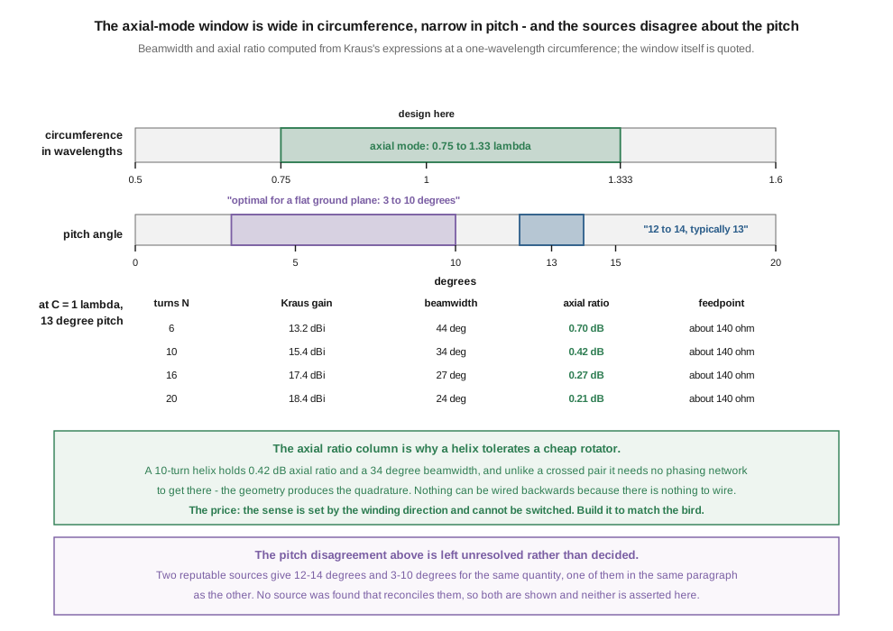
Axial mode is a window, not a resonance, and the width of the window is the helix’s best practical property.

Circumference: 0.75 to 1.33 λ. Outside that range the helix reverts to normal mode at the low end and breaks up at the high end. Inside it, the antenna works — which is why a helix is a genuinely broadband antenna, covering nearly an octave, and why a 70 cm helix is also a usable 33 cm one. Design at one wavelength and there is comfortable margin both ways.

Pitch: the sources disagree, and this dive does not adjudicate. One reference states that “the helix antenna functions well for pitch angles between 12 and 14 degrees; typically the pitch angle is taken as 13 degrees”. Another gives the same formulas and then states that “the optimal pitch that maximizes the gain for a flat ground plane is in the range 3–10 degrees”. Those two ranges do not overlap. ⚠ No source was found that reconciles them, and both are shown in the figure rather than one being asserted. The seed chapter says 12–14 degrees, which matches the first source and is what the calculations here use; a reader should know that the question is not as settled as the universal repetition of “13 degrees” implies.

What the helix gives across the window, computed at a one-wavelength circumference and a 13-degree pitch:

Table 3 — What the helix gives across the window, computed at a one-wavelength circumference and a 13-degree pitch

turns	gain (Kraus bound)	half-power beamwidth	axial ratio	feedpoint
6	13.2 dBi	44°	0.69 dB	~140 Ω
10	15.4 dBi	34°	0.42 dB	~140 Ω
16	17.4 dBi	27°	0.27 dB	~140 Ω
20	18.4 dBi	24°	0.21 dB	~140 Ω

The beamwidth follows 52 / (C_λ √(N S_λ)) degrees and the axial ratio Kraus’s (2N+1)/2N. Both are the same kind of approximation as the gain expression and should be read the same way.

⭐ The axial-ratio column is the argument for the helix, and it should be read against §3’s table rather than against another helix. A ten-turn helix holds 0.42 dB with no phasing network at all. The best a quarter-wave-fed crossed Yagi pair manages is whatever the cable impedance permits — perfect if 50 Ω line is used, 3.52 dB if 75 Ω is — and the difference between those two outcomes is a decision a builder makes, correctly or incorrectly, at the bench. The helix has no such decision to get wrong, and for an antenna that will be built once and left on a mast for ten years that is worth more than a decibel of gain.

3.9 DIY — a crossed 2 m / 70 cm array

A buildable tracked array for the FM and linear birds: crossed Yagi pairs for both bands on one cross-boom. The per-element mechanics are the Yagi-Uda dive’s; the new work is the crossing and the phasing, and §3 has already found where the published advice goes wrong.

Design. Use a published satellite-Yagi design — the WA5VJB “Cheap Yagi” and the DK7ZB crossed-Yagi notes are the community references the seed chapter names — for roughly 6 elements on 2 m and 10 on 70 cm, per plane. Cut two identical Yagis per band and mount them 90 degrees apart on a common boom.

Phasing, corrected. This is the section the seed gets wrong, and §3 gives the replacement:

1. Feed one Yagi of each pair directly.
2. Feed the other through an electrical quarter-wave of 50 Ω coax — length 0.25 λ × velocity factor. Not 75 Ω. On elements matched to 50 Ω, 50 Ω line gives exactly equal currents and therefore an axial ratio limited only by the antennas; 75 Ω line gives 3.52 dB.
3. The junction of the two branches sits at 25 Ω. Restore 50 Ω with a quarter-wave transformer of about 35 Ω — in practice two equal lengths of 75 Ω coax in parallel, which make 37.5 Ω and, evaluated as drawn, present 56.25 Ω to the feeder: an SWR of 1.125:1.
4. Choke the feeder at the antenna. The BALUNs and UNUNs dive covers the winding; common-mode current on a CP array corrupts the axial ratio specifically, which is the property the whole crossing exists to produce.

Bill of materials, per band, for two Yagis. ⚠ Prices are estimates, not quotations; nothing in this list was priced against a vendor for this dive.

Table 4 — 9. DIY — a crossed 2 m / 70 cm array

part	specification	note
element stock	⅛″–³⁄₁₆″ aluminium welding rod, or ½″ tube	per the chosen design
boom	1″ square aluminium	length per design
element mounts	insulated, commercial or printed
delay line	λ/4 of 50 Ω coax	the correction in §3 — not 75 Ω
transformer	two equal λ/4 lengths of 75 Ω in parallel	37.5 Ω; gives 1.125:1
choke	FT240-31, per plane	not optional on a CP array
connectors, hardware	N or SMA, stainless

⚠ An alternative worth pricing before building. The seed’s BOM offers a hybrid coupler as a $90 line item against $10 of coax. §4 shows what the hybrid buys — switchable sense, worth up to 21.8 dB on a bird whose sense was guessed wrong, plus correct quadrature across a band rather than at a point. On an array that will be up for years, that is one of the better-value items in the whole station, and the $10 option is a false economy for any station working more than one bird.

Tuning. Sweep each plane independently before combining; see the NanoVNA dive. Expect each Yagi to read near 1:1 alone, the paralleled pair to read about 2:1 before the transformer, and about 1.1:1 after it. Those three readings in that order are the evidence the phasing network is built correctly, and the middle one is the check the seed chapter’s procedure has no way to make. Mount the finished cross-boom balanced about the elevation axis — Vol 5 explains why that is a load-bearing requirement and not tidiness.

3.10 DIY — a 70 cm axial-mode helix

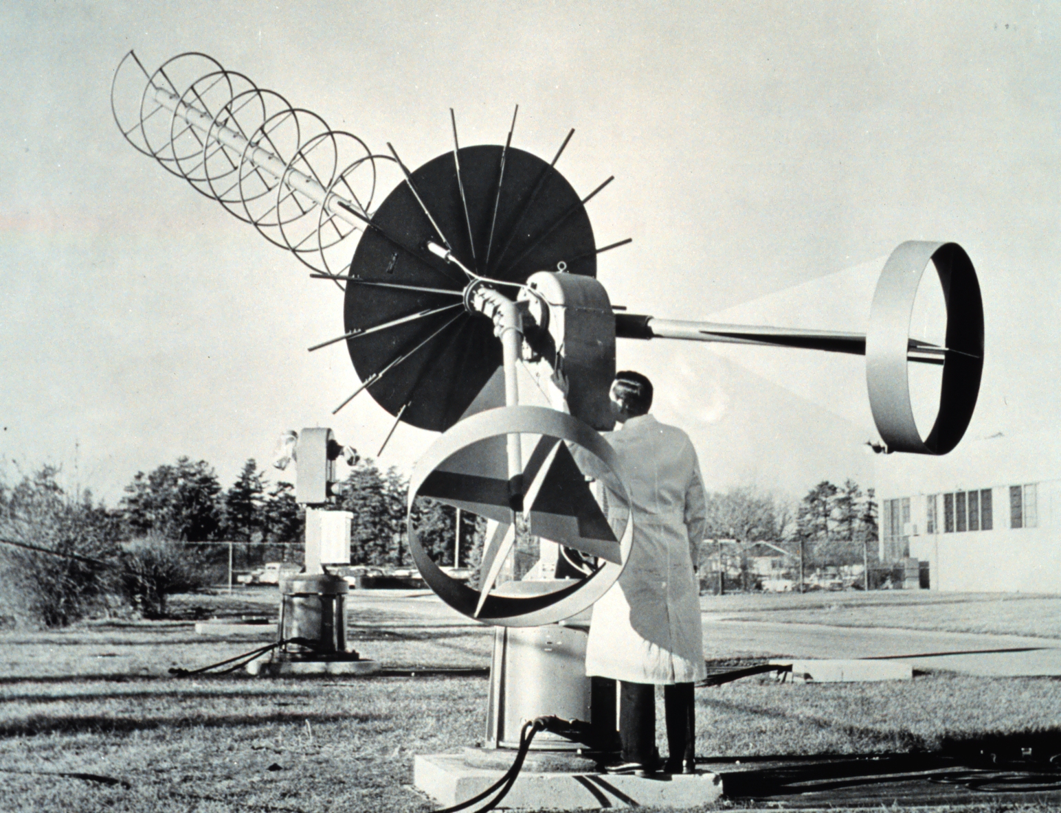
A ten-turn helix for 435 MHz gives §8’s numbers: a Kraus bound of 15.4 dBi to be read as a ceiling, about 34 degrees of beamwidth, and 0.42 dB of axial ratio. At 435 MHz one wavelength is 689 mm.

Table 5 — 10. DIY — a 70 cm axial-mode helix

parameter	value	from
circumference	689 mm (1 λ)	the centre of the axial-mode window
helix diameter	219 mm	C/π
pitch angle	13°	§8, with the caveat there
turn spacing	159 mm (0.231 λ)	C · tan 13°
turns	10
axial length	1,590 mm	N × spacing
ground plane	≥ 0.8 λ across, so 550 mm	a flat plate or a cup
feedpoint	~140 Ω	140 · C_λ

Construction. Wind the conductor on a non-conductive former — a length of drainpipe works — or support it on radial insulating spokes from a central mast. Copper tube or heavy wire; the conductor diameter is not critical in axial mode, which is part of what makes the helix a forgiving build. The ground plane goes at the feed end, and a cup or a rim of a few centimetres improves the pattern over a flat plate.

Matching. The 140 Ω feedpoint needs bringing to 50 Ω. The standard solution is not a transformer but a tapered impedance match at the first half turn — the conductor is flattened into a strip running close to the ground plane for the first 180 degrees, which presents a low impedance at the connector and transitions smoothly to the helix’s own. It is the least intuitive part of the build and the part most worth copying exactly from a published design rather than improvising. A quarter-wave transformer of √(140 × 50) = 83.7 Ω is the alternative and is easier to get right, at the cost of bandwidth — which partly defeats the purpose of choosing a helix.

Sense. Decide it before winding, and check it against the drawing before the former comes out. A right-hand wound helix — advancing away from the feed, turning clockwise as seen from behind — radiates RHCP. §6: it cannot be changed afterwards.

Testing. Sweep it. A correct axial-mode helix shows a broad, shallow return-loss curve across a very wide band with no sharp feature; a sharp resonance means it is not in axial mode. ⚠ Neither the axial ratio nor the sense can be verified with a VNA, and this dive has no first-hand procedure for either — the same gap Vol 2 §9 records for the quadrifilar helix, and for the same reason.

3.11 Buys, dated

Everything here was checked on 17 September 2026. Figures that could not be verified are marked as unverified rather than filled in.

3.11.1 Verified

Table 6 — Verified

product	what it is	verified figure
M2 2MCP8A	crossed Yagi, 143–147 MHz, 9.2 dBic, 60° circular beamwidth, 64″ boom, 0.5 sq ft wind area, 4 lb	$367.95
M2 436CP16	crossed Yagi, 432–438 MHz, 13.3 dBic, 42° circular beamwidth, 65¾″ boom, 0.4 sq ft, 4 lb	$367.95
M2 LEO Pack (FGLEOPACK)	the two above plus an 8½ ft cross boom	$723.99
Elk 2M/440L5	handheld dual-band log-periodic, linear	$137.95–$170.95
Arrow II 146/437-10	handheld, 3 el on 2 m crossed with 7 el on 70 cm, 37½″ boom	price not published on the product page

🔴 The seed chapter’s price for the LEO Pack is wrong by 31 to 81 per cent. It lists the “M2 Antenna LEO-Pack (2MCP8A + 436CP16/30)” at $400–550; the verified figure is $723.99.

⭐ And the pack is worth buying rather than the antennas separately, which falls out of the same check: two antennas at $367.95 each come to $735.90, so the pack is $11.91 cheaper and includes the cross boom. That is a small saving and a real one, and it is the kind of thing a dated price table exists to surface.

⚠ The wind-area and boom figures above are the numbers Vol 5 sizes a rotator with, and they are worth noting as the more useful half of this table. A crossed Yagi’s gain is on every listing; its wind area is on very few, and it is the quantity that decides whether a rotator survives.

3.11.2 Unverified, and recorded as such

The Arrow II’s price could not be established. The manufacturer’s product page carries the element counts, the boom length and the power ratings — 10 W hand-held, 150 W mounted away from people — but no price, and the pricing page could not be retrieved. The seed’s “$130–160” is plausible and is not repeated as a verified figure.

“M2 Antenna 2MCP22 / 436CP42UG, $300–600 each” could not be checked. ⚠ Given that the two M2 antennas that were checked are $367.95 each, a bracket topping out at $600 for the larger models is not obviously wrong; it is simply not verified.

“WiMo / Diamond crossed Yagis, $200–400” could not be checked; WiMo’s site refused retrieval.

The “SP-70 / ARR” hybrid coupler — §3. The device class is real; the designation could not be matched to a product and is withdrawn.

3.11.3 What to avoid, which the seed gets right

Its two warnings both survive and this dive can now supply the mechanisms:

• “‘Satellite’ Yagis sold without specifying CP sense or axial ratio.” Correct, and Vol 1 §5 and §6 put numbers on both halves: the sense is worth up to 21.8 dB and the axial ratio decides how much of that is real, and a listing giving neither has described the antenna’s polarization not at all.
• “Undersizing the rotator.” Correct, and Vol 5 computes it from the wind-area figures in the table above.

To those, §3 adds a third that the seed does not have: a crossed Yagi sold or built with a 75 Ω quarter-wave phasing line on 50 Ω elements has a 3.5 dB axial ratio by construction, whatever its listing claims. If a vendor publishes the phasing arrangement, it can be checked with the arithmetic in §3.

3.12 Resources

• Kraus, Antennas — the axial-mode helix: the gain, beamwidth and axial-ratio expressions used in §7 and §8, and the axial-mode window.
• ⚠ The statement that the Kraus gain expression overestimates real helix gain by several decibels is well attested in general references. §7 records that a specific measured deficit against turn count could not be verified for this dive and is therefore not given.
• M2 Antenna Systems (m2inc.com) — the 2MCP8A, 436CP16 and LEO Pack specifications and prices in §11, read 17 September 2026.
• Elk Antennas (elkantennas.com) and Arrow Antennas (arrowantennas.com) — the handheld beams of §5, read 17 September 2026.
• DK7ZB and WA5VJB — the published crossed-Yagi and “Cheap Yagi” designs §9’s build leans on.
• Yagi-Uda antennas — the parasitic-array theory this volume assumes, and the element mechanics §9’s build needs.
• Vol 1 — the polarization loss that makes §4’s relay worth its price, and the gain bound that makes §2’s argument.
• Vol 2 — the fixed antennas, and the same phasing arithmetic applied to a turnstile.
• Vol 4 — the helix as a dish feed, and the preamp that belongs behind any of these antennas.
• Vol 5 — the rotator that carries the array, sized from §11’s wind-area figures.
• BALUNs and UNUNs — the choke §9 fits, and why its absence corrupts the axial ratio without disturbing the SWR.
• Satellite tracking — pass prediction, and the software that drives the rotator this volume’s arrays sit on.