Why a Cone Is Wideband

---

1.1 About this volume

The discone is the most widely owned and least examined antenna in this hub. It is what comes in the box with a scanner, what sits on the roof of every monitoring site, and what almost every wideband SDR in the peer projects is eventually connected to. It is also an antenna whose behaviour is unusually easy to compute — its defining property is that its shape is specified by an angle, and an angle is the only parameter it has — and that combination, ubiquity plus computability, is why the previous edition of this chapter turned out to contain so much that can be checked and so much that does not survive checking.

This dive covers the geometric wideband family: the discone proper, the symmetric biconical, the conical monopole over a ground plane, the sleeve, and the planar bow-tie. What these have in common is that their bandwidth comes from the shape of a cone. The other wideband family — the log-periodic dipole array, the horn, the equiangular spiral, the Vivaldi — gets its bandwidth from a repeating structure rather than from a smooth taper, has a directional pattern rather than an omnidirectional one, and is a separate dive.

Three results from this volume run against what the previous edition says, and they are worth stating before the reasoning rather than after it.

The first is that the chapter uses one word, “bandwidth”, for two quantities that have different limits, different mechanisms and different numbers. A discone’s impedance bandwidth and its pattern bandwidth are not the same interval and do not end for the same reason. §2 separates them, and the separation is this dive’s organising idea. The chapter half-sees it — it notices that vendors quote one range for receive and a narrower one for transmit — but attributes the difference entirely to standing-wave ratio, which is the wrong mechanism at both ends.

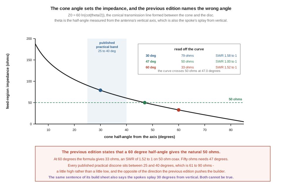
The second is an angle stated at twice its value. The chapter specifies a 60° cone half-angle throughout, calls it the standard, and builds its DIY antenna around it. Computed from the conical-line formula, a 60° half-angle is a 33 Ω antenna, not the 50 Ω the chapter claims; 50 Ω needs 47°; and every published practical discone sits between 25° and 40°, which is 61 to 90 Ω. §5 shows that the chapter’s own build sheet contains the correct angle as well, in the same sentence, and that the two readings differ by a factor of 1.73 in the cone’s base diameter.

The third is that the number on the front of every scanner discone box is not an antenna cutoff at all. Five commercial discones were checked against their makers’ own published dimensions on 17 September 2026. Every one of them advertises a receive floor of 25 MHz — and a quarter wave at 25 MHz is 3.00 m, against a tallest published overall height of 1.70 m. §6 works this out. The antennas are not lying; they are answering a different question, and the answer they give to the other question — their published transmit floor — lands within a few per cent of where the physics puts the real edge.

1.2 Two bandwidths, and one word for both

The chapter’s §8 is titled “the 10:1 bandwidth claim, examined”, and its examination reaches a conclusion worth quoting because most of it is right:

The vendor spec’s 40:1 claim is honest for receive; the transmit usable range is 10:1.

⭐ The insight is correct and it is the best thing in the chapter. A discone really is sold with two ranges; the wider one really is a receive figure; and the reason really is that receive tolerates a mismatch that transmit does not. Nothing in this dive disturbs that framework, and it would be an over-correction to treat the passage as an error.

What does not survive is every number in it and the mechanism underneath it.

The numbers. Diamond publishes the D130J as 25–1300 MHz on receive and 50–1300 MHz on transmit. That is 52:1 and 26:1, not 40:1 and 10:1. The D3000N is 25–3000 and 50–3000: 120:1 and 60:1. The MFJ-1868 is 25–1300 and 50–1300, the same 52:1 and 26:1. The chapter’s “10:1” for the transmit range understates the manufacturers’ own transmit claims by a factor of two and a half, and its “40:1” for the receive range understates them too. This is a rare direction for a correction in this program — the chapter is being more conservative than the evidence, not less — and it matters because the conservatism hides the actual structure.

The mechanism is the part that is wrong. The chapter’s account of why the two ranges differ is a table of standing-wave ratio degrading smoothly with frequency:

• 30 MHz – 300 MHz: SWR < 2:1, full performance
• 300 MHz – 600 MHz: SWR 2:1 to 3:1, mild degradation
• 600 MHz – 1000 MHz: SWR 2.5:1 to 4:1, noticeable degradation
• 1000 MHz – 1300 MHz: SWR 3:1 to 5:1, significant degradation

🔴 That describes a match that gets steadily worse as frequency rises, which is the opposite of how this geometry behaves. The whole reason a cone is used is that its impedance is insensitive to frequency once the structure is large enough to radiate — §4 derives why — and the consequence is that a discone’s match is worst at the bottom of its range, where the antenna is electrically small, and good essentially everywhere above that. Wikipedia’s account, sourced to the ARRL Antenna Book and to Paul Lee’s vertical-antenna handbook, puts it as “SWR is typically 1.5:1 or less over several octaves of frequency.” The degradation the chapter tabulates at the top of the band is not primarily a match failure.

So the two bandwidths need naming separately, and each needs its own limit:

Impedance bandwidth ends at the bottom, and it ends because of truncation — the cone runs out of length and the antenna stops being electrically big enough to look like the infinite structure the formula describes. §6 puts a hard bound on that frequency from published dimensions alone.

Pattern bandwidth ends at the top, and it ends while the match is still fine. The structure becomes many wavelengths tall, the single horizon-directed lobe cannot survive that, and the energy goes somewhere the listener is not. §7 states the bound and Vol 3 computes it.

Once those are separated, the two-floor convention on every product page stops looking like marketing and starts looking like an engineering statement, which is what §6 argues it is.

1.3 What Rumsey’s principle says, and what a discone actually obeys

The chapter opens its theory section with Rumsey, and the framing is broadly sound:

Victor Rumsey (1957) proved that any antenna whose geometry is defined entirely by angles (no characteristic length) is frequency-independent.

Two things need saying about this, one bibliographic and one substantive.

⚠ The citation could not be verified and has been replaced rather than repeated. The chapter’s resources list gives “Rumsey 1957 paper (‘Frequency Independent Antennas,’ IRE National Convention Record)”. A 1957 convention-record paper of that name is very widely cited in the secondary literature, and it may well be exactly right — but it could not be confirmed against any primary or bibliographic source available to this dive, and this program’s rule is that an unverifiable citation is withdrawn rather than softened. What can be verified is Rumsey’s book, Frequency Independent Antennas, Academic Press, New York and London, 1966, which is the citation the log-periodic literature actually carries. This dive cites the book.

The substantive point is more interesting, and the chapter gets it half right in a way that matters.

A cone does obey the angle-only condition. A discone does not. The distinction is the whole reason a discone has band edges at all, and the chapter’s own later sections depend on it without ever connecting them to this paragraph.

Consider what the condition requires. An antenna is frequency-independent if scaling the whole structure by any factor maps it onto itself — which means it can have no dimension with units of length, because any such dimension would pick out a frequency. An infinite cone satisfies this: it is specified by one angle and extends forever. Wikipedia’s biconical article states the consequence directly — for a theoretical infinite antenna “the characteristic impedance at the point of connection is a function of the cone angle only and is independent of the frequency.”

A real discone has at least three lengths in it. The cone has a slant height, because it stops. The disc has a diameter. And the feed region has a gap. Each of those is a length, each picks out a frequency, and together they are the band edges. The structure is not frequency-independent; it is frequency-independent in its middle, over the interval where the cone is long enough for the terminating truncation to be far away in wavelengths and short enough that the disc is not yet many wavelengths across.

⭐ The chapter knows all three of these lengths. Its §8.3 lists exactly them, as “bandwidth degradation modes” — slant height at the lower bound, disc-to-cone spacing at the upper, plus structural resonances. What it never does is notice that they are the same facts as its Rumsey paragraph, seen from the other side. The band edges are not an unfortunate practical departure from the theory. They are what the theory predicts the moment you build a finite object, and every one of them can be located from the antenna’s dimensions.

The chapter’s list of angle-defined examples is worth endorsing rather than fixing. A cone, a biconical structure and an equiangular spiral all qualify, and its instinct that these belong to one family is right — it is the same instinct that puts the log-periodic and spiral antennas in the companion dive. The one entry that needs a footnote is the discone itself, which appears in the family on the strength of its cone while carrying a disc that disqualifies it.

1.4 The cone is a transmission line, and its angle is its impedance

The chapter’s §2.3 offers the right mechanism and then states it backwards:

The discone’s wideband behavior comes from the tapered transmission line that the cone forms. The cone’s characteristic impedance varies along its length: high at the tip, low at the base. This impedance taper acts as an impedance-matching transformer that gives a smooth Z presentation across frequency.

🔴🔴 The first sentence is exactly right and the second destroys it. A conical transmission line is the one taper whose characteristic impedance does not vary along its length, and that constancy is precisely why the geometry is wideband. If the impedance varied from tip to base, the structure would have a length scale, would not be self-similar, and would not be frequency-independent in the sense §3 just established. The chapter’s own Rumsey paragraph, two sections earlier, says so.

The mechanism, stated correctly: a spherical TEM wave travelling outward from the apex between the cone and the disc sees, at every radius, the same angular geometry. The two conductors subtend fixed angles; the radius scales out. So the wave impedance it encounters is a constant, set by the angles alone:

Z₀ = 60 · ln( cot(θ/2) )

where θ is the cone’s half-angle measured from the antenna’s vertical axis. The disc plays the part of the image plane — the degenerate cone at 90°, whose cot(45°) = 1 contributes nothing — which is why the discone takes the factor of 60 and the symmetric biconical, two cones tip to tip with no ground plane, takes twice it:

Z₀ = 120 · ln( cot(θ/2) )

Evaluated across the practical range, with the resulting standing-wave ratio on 50 Ω coax:

Table 1 — Evaluated across the practical range, with the resulting standing-wave ratio on 50 Ω coax

cone half-angle	discone Z₀	SWR on 50 Ω	biconical Z₀
20°	104 Ω	2.08:1	208 Ω
25°	90 Ω	1.81:1	181 Ω
30°	79 Ω	1.58:1	158 Ω
35°	69 Ω	1.39:1	139 Ω
40°	61 Ω	1.21:1	121 Ω
47°	50 Ω	1.00:1	100 Ω
60°	33 Ω	1.52:1	66 Ω
75°	16 Ω	3.14:1	32 Ω

Three things fall out of that table, and all three contradict something the chapter prints.

The 50 Ω point is at 47°, not 60°. The chapter asserts “60° gives ~50 Ω” in four separate places, including the caption of its geometry diagram and the first line of its DIY build table.

Practical discones are a little high in impedance, not a little low. Wikipedia gives the published practical range as “The cone angle is generally from 25 to 40 degrees”, which the table puts at 61 to 90 Ω. The chapter’s own impedance table agrees with this in direction — it too shows impedance falling as the cone widens — and even gets close to the right values at the narrow end, listing 80–100 Ω for a 30° cone against the formula’s 79 Ω. ⭐ That is worth recording as confirmed rather than corrected, because it means the chapter’s table is not invented; it is the right function evaluated at shifted arguments, and the shift is the same factor-of-two angle confusion §5 takes apart.

The 60° figure is not catastrophic, which is why it survived. A 33 Ω antenna on 50 Ω coax is 1.51:1, and no one operating a scanner would notice. The error does not announce itself in a sweep; it announces itself in a cone twice as wide as it should be, which is a mechanical and wind-loading problem before it is an electrical one.

1.4.1 A measurement, from a photograph

There is one independent check available without a bench. The solid-copper discone photographed for Wikimedia Commons is a clean, unobstructed side view of a real antenna, and its silhouette can be measured.

Fitting a straight line by least squares to 214 samples of the cone’s left edge — the left edge only, because the right is contaminated by the background — gives a slope of dx/dy = −0.501, and therefore a cone half-angle of 26.6°.

⚠ That is a close-up photograph and perspective inflates near dimensions, so the figure carries a few degrees of uncertainty and its implied 87 Ω should not be read as this antenna’s feedpoint impedance — the infinite-cone formula describes the feed region, not a truncated antenna’s terminals. What the measurement establishes is robust to all of that: the cone on a real discone splays at somewhere around a quarter turn of a right angle from vertical, not two thirds of one. It sits squarely inside the published 25°–40° band and nowhere near 60°.

1.5 Sixty degrees, thirty degrees, and the cone that is specified twice

The chapter’s construction section contains this sentence:

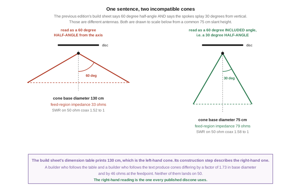
Assemble the cone. Attach 12 cone spokes radially at the apex hub. The spokes splay outward at 30° from vertical (60° half-angle).

🔴 The splay from vertical is the half-angle. They are the same measurement of the same thing: the angle between a spoke and the antenna’s axis. The parenthesis does not restate the figure, it doubles it. What has happened is a conflation of the half-angle with the included apex angle — the full angle from one spoke across to the spoke opposite, which for a 30° half-angle is indeed 60°. Both numbers are in the sentence; only one of them is a half-angle.

This would be a vocabulary slip if it stayed in one sentence. It does not. The chapter’s dimension tables are computed from the 60° reading, and its construction steps describe the 30° one, so the two halves of the same build sheet describe different antennas.

Taking the chapter’s own 75 cm cone slant and its own stated relation base diameter = 2 × slant × sin(half-angle):

Table 2 — Taking the chapter's own 75 cm cone slant and its own stated relation base diameter = 2 × slant × sin(half-angle)

	as the table computes it	as the text describes it
half-angle	60°	30°
cone base diameter	130 cm	75 cm
feed-region impedance	33 Ω	79 Ω
SWR on 50 Ω	1.52:1	1.58:1

The chapter’s build table prints 130 cm, which is the left-hand column. Its construction step describes the right-hand one. A builder who works from the table and a builder who works from the text produce cones differing by a factor of 1.73 in base diameter and by 46 Ω at the feedpoint — and, in the pleasing symmetry that explains why neither party ever discovers the problem, the two land at almost identical standing-wave ratios on opposite sides of 50 Ω. Both builds work. Neither matches the chapter’s claim, and the two are not the same antenna.

The same doubling propagates upward into the chapter’s worked examples. Its 30–300 MHz discone is given a “cone base diameter: ~4.3 m at 60° half-angle”; at the 30° the construction section would have specified, it is 2.5 m. A 4.3 m cone is a genuinely large structure to put on a roof, and it is 1.73 times larger than the antenna the chapter thinks it is describing.

⚠ The right-hand reading is the correct one. It is what Wikipedia’s 25°–40° range describes, what the photograph in §4 measures at 26.6°, and what produces a cone of a size anyone has ever actually built. The chapter’s tables, not its prose, are what need changing.

1.5.1 Where the 60° may have come from

This is worth a paragraph because it is not a random error and the same trap is available to any reader. Antenna literature quotes cone angles in at least three conventions: the half-angle from the axis, the included apex angle, and occasionally the angle from the horizontal — which is the complement of the half-angle and therefore turns 30° into 60° by a different route. Wikipedia’s own sentence, “The cone angle is generally from 25 to 40 degrees”, does not say which convention it uses; the number only resolves to the half-angle because the impedance formula and the photographs agree that it must.

⭐ The general rule this dive adopts as a result: a cone angle quoted without its reference is not a specification. Every angle in the four volumes that follow is stated as a half-angle from the axis, and every figure that draws a cone draws it to scale so the drawing itself carries the convention.

1.6 What sets the bottom, and the number on the box

Here is the arithmetic the chapter never does.

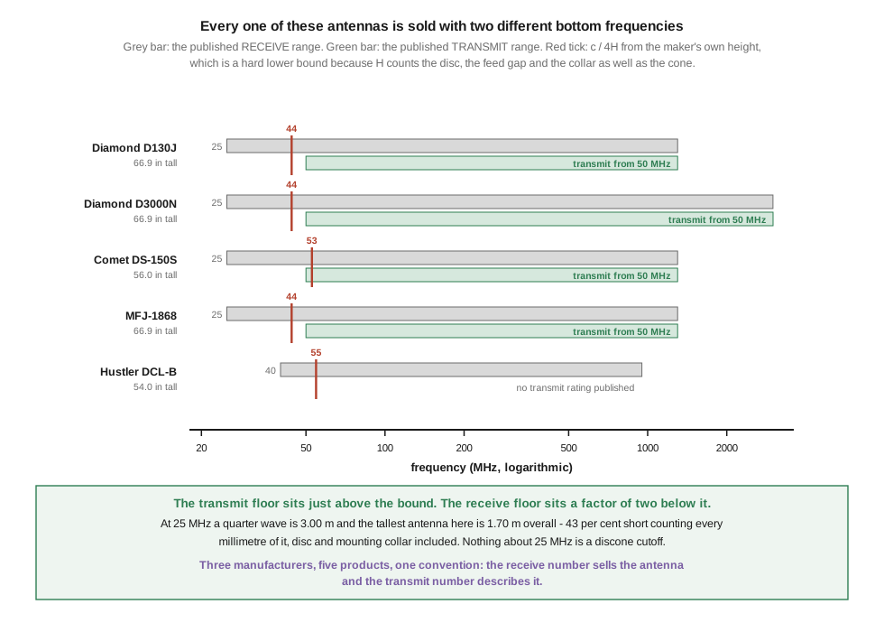
A structure of overall height H cannot present a quarter wave at any frequency below f = c / 4H. This is a bound, not a fit, and it is a generous one, because a manufacturer’s published height includes the disc, the feed gap, the insulator and the mounting collar as well as the cone that does the radiating. The real cone is shorter than H, so the real cutoff is above the bound.

Five discones, with specifications and prices read from the makers’ own listings on 17 September 2026:

Table 3 — Five discones, with specifications and prices read from the makers' own listings on 17 September 2026

antenna	published height	c / 4H	published RX floor	published TX floor
Diamond D130J	66.9 in (1.70 m)	44.1 MHz	25 MHz	50 MHz
Diamond D3000N	66.9 in (1.70 m)	44.1 MHz	25 MHz	50 MHz
Comet DS-150S	56.0 in (1.42 m)	52.7 MHz	25 MHz	50 MHz
MFJ-1868	66.9 in (1.70 m)	44.1 MHz	25 MHz	50 MHz
Hustler DCL-B	54.0 in (1.37 m)	54.6 MHz	40 MHz	not published

⭐⭐ Three manufacturers, five products, one convention. The published transmit floor sits just above the bound the antenna’s own height permits; the published receive floor sits a factor of two below it.

Take the Diamond D130J. At its transmit floor of 50 MHz a quarter wave is 1.50 m, against 1.70 m of antenna — consistent, with 20 cm left over for the disc, the gap and the collar, which is about what the photographs show those parts occupying. At its receive floor of 25 MHz a quarter wave is 3.00 m, and the entire antenna, counting every millimetre of it, is 43 % short of that. There is no reading of the geometry on which 25 MHz is a cutoff. The Comet DS-150S is the tightest case of the five and confirms the pattern from the other side: its bound is 52.7 MHz and its published transmit floor is 50 MHz, so its cone is using essentially the whole of its height.

So what is the 25 MHz? It is an honest statement about a regime rather than about a resonance, and the chapter very nearly says so. At 25 MHz the D130J is a 0.14 λ stub with a large capacitive top hat: badly mismatched, inefficient, and entirely usable, because reception below roughly 30 MHz is limited by external noise arriving through the antenna rather than by the receiver’s own noise floor. The receive-only loops dive establishes that case in full, and its conclusion applies unchanged here — attenuating the wanted signal and the noise arriving with it by the same amount does not change the ratio between them, so a mismatch that would be intolerable on transmit costs the listener nothing.

The chapter states this correctly in principle and slightly wrongly in arithmetic:

For receive applications, SWR up to 4:1 is acceptable (mismatch loss < 1.5 dB, no impact on noise figure).

The principle is right and is confirmed. The number is not: at 4:1 the reflection coefficient is 0.600 and the mismatch loss is −10 log₁₀(1 − 0.36) = 1.94 dB. The chapter’s 1.5 dB corresponds to about 3.4:1. ⚠ This is a correction of half a decibel to a claim whose conclusion is unaffected, and it is recorded in that spirit: 1.94 dB of mismatch loss is still nothing against the tens of decibels of external-noise margin that make the regime work.

⚠ One thing cannot be settled here and is left open rather than filled in. No manufacturer among the five publishes a standing-wave curve, and none publishes the SWR its antenna actually presents at 25 MHz. The chapter’s tabulated SWR figures across the band have no visible source and are not reproduced in this dive. What the discone’s match really does below its cutoff is a bench question, and Vol 5 is written as the procedure that answers it.

1.7 What sets the top, and why it is not the match

The upper end is the reverse situation: the impedance stays good and the antenna stops being useful anyway.

The arithmetic is immediate from the same heights. The D130J’s 1.70 m structure is 7.4 wavelengths tall at its published 1300 MHz ceiling. The D3000N’s identical 1.70 m structure is 17.0 wavelengths tall at 3000 MHz. Nothing about a radiating structure seventeen wavelengths tall keeps a single lobe pointed at the horizon.

This is what the published accounts describe. Wikipedia, on the discone at the top of its range: “The elevation pattern might be distorted with grating lobes.” That is a pattern statement, not an impedance statement, and the word “grating” is the right one — a structure many wavelengths long with current distributed along it radiates into multiple lobes for the same reason a diffraction grating produces multiple orders.

The chapter’s account of the upper limit is the one part of its §8.3 that is a real effect stated in the right place:

Upper bound: the disc-to-cone spacing becomes too large relative to wavelength (the gap region becomes a transmission line of significant length)

⭐ That is correct, and it is the mechanism that limits the impedance. The feed gap is one of §3’s three lengths, and when it stops being electrically small the feed stops behaving as a point and the match does finally degrade. What the chapter does not do is notice that this happens later than the pattern failure, so it is not what ends the antenna’s usefulness. A discone whose match has survived to 1300 MHz has long since stopped putting its energy where a listener at ground level is standing.

⚠ The size of that effect is Vol 3’s subject and is not asserted here. The pattern computation needs care — a discone is not a thin monopole, and the obvious model for the lobe structure is not obviously the right one — so this volume states the bound and the mechanism and leaves the numbers to the volume that can compute them properly.

What the separation buys, immediately, is a better way to read a specification. A discone quoted as “25–3000 MHz” is making three claims at once: that it will present a tolerable match over most of that span, which is probably true; that it will hear something at the bottom of it, which is true for a reason that has nothing to do with the antenna being resonant; and that the energy at the top of it is going somewhere useful, which is the claim nobody checks.

1.8 Where this volume hands off

The foundation is in place, and it is mostly a matter of having separated things the chapter runs together.

A cone is wideband because a conical transmission line has the same characteristic impedance at every radius — not, as the chapter says, because its impedance tapers from tip to base. That impedance is 60 ln(cot(θ/2)) for a discone and twice that for a symmetric biconical, and it is a function of one angle and nothing else. The angle that gives 50 Ω is 47°; the angle every practical discone uses is between 25° and 40°, giving 61 to 90 Ω; and the 60° the chapter specifies throughout gives 33 Ω and is the included apex angle of a 30° cone wearing a half-angle’s label — in a build sheet that states both readings in one sentence and computes its dimension table from the wrong one.

A finite discone is not frequency-independent, because it has three lengths: a cone slant, a disc diameter and a feed gap. The first sets the bottom, the last eventually spoils the match at the top, and the second is what the pattern founders on first. The bottom can be bounded from published dimensions alone, and doing so finds that every scanner discone on the market is sold with two bottom frequencies — a transmit floor that sits just above the bound, and a receive floor a factor of two below it that is a statement about the noise regime rather than about the antenna.

From here:

• Vol 2 — The discone proper takes the geometry to construction depth: the disc-to-cone ratios and which of them the published rules actually specify, the feed gap, spoked against solid, and how many spokes a cone needs before it stops behaving as a cone.
• Vol 3 — The pattern takes §7’s bound and computes it, and takes up the claim this dive most expects to have to correct: the chapter states that a discone peaks at 25–35° of elevation and is weak at the horizon, which is the reverse of the published accounts.
• Vol 4 — The rest of the family covers the symmetric biconical, the conical monopole, the sleeve and the bow-tie, including the EMC-test world where biconicals are calibrated instruments rather than scanner accessories — and where the chapter’s product list needs the most work.
• Vol 5 — Build, measure and buy builds a discone with the angle corrected, replaces a verification procedure that cannot fail, and gives a commercial survey with a date on it.

Two items are owed against this volume and are recorded rather than skipped. No measurement in this dive is first-hand; the photograph measured in §4 is the closest thing to one, and it is a photograph. And the Rumsey 1957 citation remains unresolved — the 1966 book is verified and is what this dive cites, but a reader with access to the IRE convention records could settle the earlier paper in ten minutes and it would be worth doing, because the chapter’s date is probably right.

1.9 Resources

• Armig G. Kandoian, Broad band antenna, US Patent 2,368,663 — filed 15 May 1943, granted 6 February 1945, assigned to the Federal Telephone and Radio Corporation. The primary source for the discone, and the document Vol 2 uses in place of the chapter’s unverifiable paper citation.
• V. H. Rumsey, Frequency Independent Antennas, Academic Press, New York and London, 1966 — the angle-only condition §3 rests on, cited from the book because the 1957 convention paper could not be verified.
• Paul Lee, The Amateur Radio Vertical Antenna Handbook, 2nd ed., CQ Communications, 1996, pp. 50–51 — one of the two sources behind the published 25°–40° cone-angle range and the 0.7 disc ratio.
• Jerry Hall, ed., The ARRL Antenna Book, 16th ed., 1991, pp. 7–17 — the other, and the standard amateur treatment of the discone family.
• Diamond Antenna, Comet, MFJ Enterprises and Hustler published specifications — the five antennas in §6, read from manufacturer and dealer listings on 17 September 2026. Vol 5 carries the full survey with prices.
• Receive-only loops, Vol 1 — why loss is free when external noise sets the floor, which is the argument that makes §6’s receive floor an honest specification.
• Log-periodic and structured wideband antennas — the directional half of the wideband problem, and the antennas that get their bandwidth from a repeating structure rather than a smooth taper.
• Antenna theory and practice — impedance, reflection coefficient, mismatch loss and pattern vocabulary, if any of §6’s arithmetic needs shoring up.
• NanoVNA, Vol 4 — the sweep technique Vol 5 uses to answer the question §6 leaves open.