The Discone Proper

---

2.1 About this volume

Vol 1 established the one parameter that matters — the cone’s half-angle, which sets the impedance and which the previous edition of this chapter states at twice its value. This volume takes the rest of the geometry to the depth a builder needs, and it is mostly a volume about reference dimensions: about ratios that are quoted without saying what they are ratios of.

That turns out to be the characteristic failure of the discone literature, and it is a more interesting failure than plain error. A discone is specified almost entirely by ratios — disc to cone, gap to something, spoke count to something else — and because the antenna is forgiving, a ratio read against the wrong reference dimension produces an antenna that still works. Nobody finds out. The rules propagate, each restatement slightly further from whatever the original measurement was, and the chapter under review contains at least three of them.

Three results carry the volume.

The founding patent contains no dimensions at all. §2 reads it. The chapter attributes the canonical geometric relationships to Kandoian’s original work; the patent establishes none of them, says the disc “may be either round, square, or of other configuration”, and was filed for an entirely different application than the one the chapter describes. Two of the chapter’s four historical claims are wrong and a third could not be verified.

The two disc rules in circulation differ, and coincide at exactly one angle. §3 computes it. “Disc diameter = 0.7 × cone slant” and “disc diameter = 0.7 × cone base diameter” are different statements; they agree when sin θ = 0.5, that is at 30.00° — the centre of the published practical band and the angle the chapter’s own construction text specifies. The ambiguity is harmless by accident, and stops being harmless the moment anyone builds the 60° cone the chapter’s tables call for.

And the required number of spokes has no frequency in it. §5 derives this, and it is the volume’s best result. The chapter ties spoke count to the top of the band — “8 spokes are adequate for 1 GHz operation; 16 spokes give cleaner pattern at the high frequency end” — which is the natural assumption and is indexed on the wrong variable. In the region of the cone that is actually radiating, the spacing between spokes measured in wavelengths is π sin θ / 2N, a constant. A twelve-spoke cone sits at 0.0654 λ between spokes at 50 MHz and at 1300 MHz alike.

2.2 What the patent says, and who actually built it

The chapter’s history is four sentences and needs three corrections. Here it is in full:

Armig Kandoian published the discone in a 1945 paper in IRE Proceedings. The geometry was developed during WWII at FCC Laboratories as a wideband VHF/UHF receive antenna for monitoring foreign communications. The original Kandoian discone used: 60° cone half-angle; disc-to-cone-slant ratio of 0.7; solid (or near-solid) cone construction; solid disc construction. The 1945 paper established the canonical geometric relationships that essentially every subsequent discone has followed.

The primary document is US Patent 2,368,663, Broad band antenna, Armig G. Kandoian, filed 15 May 1943, granted 6 February 1945, and it was read for this dive.

🔴 The 1945 date belongs to a patent, not a paper. A Kandoian paper in the Proceedings of the IRE is widely referenced in secondary accounts, and it may well exist — but the title the chapter gives it could not be verified against any primary or bibliographic source available here, and per this program’s rule it is withdrawn rather than repeated or softened. The patent is verified, is the earlier document, and is what this dive cites.

🔴 “FCC Laboratories” is a regulator, and the assignee is a manufacturer. The patent is assigned to the Federal Telephone and Radio Corporation, a maker of radio equipment later absorbed into ITT. The Federal Communications Commission neither developed nor sold antennas. The likely path of the error is visible in the name: Federal Telephone and Radio, expanded into the wrong federal body. ⭐ It is worth flagging as a class of mistake rather than a one-off, because corporate laboratories of that era carried names — Federal, General, National, Standard — that read today like government agencies and are routinely misattributed as such.

🔴 The stated application is wrong, and the correct one explains the antenna. The chapter says the discone was built for “monitoring foreign communications”. The patent’s own framing is aircraft: it describes work in “ultra-high frequency radio technique” for aircraft communication and direction finding, needing antennas that are “small and rigid” with a “minimum of wind resistance”. ⭐ That last phrase is the origin of everything §5 is about. The discone’s whole later history of spoked discs and skeletal cones descends from a requirement to present as little area to the airstream as possible — a constraint from an aeroplane, inherited by an antenna that now spends its life bolted to a chimney.

🔴 The patent establishes none of the canonical relationships. There is no cone angle in it, no disc-to-slant ratio, no relation between the cone’s length and the lowest wavelength, and no feed-gap dimension. On the disc’s shape it is explicitly permissive: “The disk may be either round, square, Ior of other configuration, but because of symmetry the round form is preferred.” On performance it claims only that the “antenna impedance is substantially constant over a wide frequency band”. So the chapter’s third sentence — the list of four specific original dimensions — has no support in the document it attributes them to, and its fourth sentence, that the paper established the canonical geometry, is false of the patent whatever a paper may have said.

⚠ Where the dimensional rules actually come from could not be settled here, and is left open rather than filled in. A 1953 Electronics design article is the usual attribution in amateur folklore; it could not be verified. What can be verified is that the two secondary works Wikipedia sources the rules to — the ARRL Antenna Book and Paul Lee’s Amateur Radio Vertical Antenna Handbook — both carry them, and those are the citations this dive uses. Tracing the rules to their measurement would be a genuine contribution and is recorded as owed.

2.3 The disc: one ratio, two reference dimensions

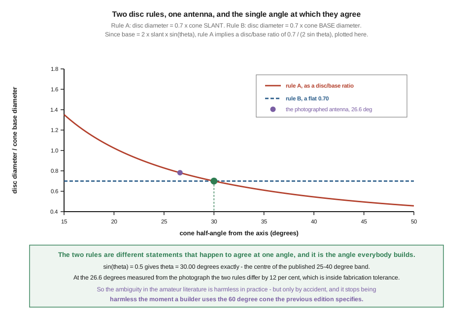
Two rules are in circulation and they are not the same rule.

Rule A, which the chapter states: “Disc diameter = 0.7 × cone slant”.

Rule B, which Wikipedia states, sourced to the ARRL Antenna Book and Paul Lee: “The disc should have an overall diameter of 0.7 times a quarter wavelength of the antenna’s lowest frequency.”

At first reading these are the same, and that is worth saying because it is the rare case in this dive where the chapter agrees with the published source. Since the cone slant is a quarter wave at the lowest frequency — the other half of the same design convention — 0.7 × slant and 0.7 × (λ/4) are the same length. ⭐ Rule A as the chapter states it is confirmed, not corrected.

The difficulty is a third form that circulates widely and reads the 0.7 against the cone’s base diameter instead. That is a different statement, because base and slant are related by the cone angle:

base diameter = 2 × slant × sin θ

so a disc specified as 0.7 × slant has a disc-to-base ratio of

0.7 / (2 sin θ)

which is a function of the cone angle and equals 0.7 only when sin θ = 0.5. Solving: θ = 30.00° exactly.

Table 1 — 3. The disc: one ratio, two reference dimensions

cone half-angle	disc/base implied by rule A	rule B asserts
20°	1.023	0.700
25°	0.828	0.700
26.6° (the measured antenna)	0.782	0.700
30°	0.700	0.700
35°	0.610	0.700
40°	0.545	0.700
60° (the chapter’s cone)	0.404	0.700

⭐⭐ The two rules agree at exactly the angle everybody builds at, which is why the ambiguity has survived in the literature for eighty years without anyone being harmed by it. At the 26.6° measured from the photograph in Vol 1 they differ by 12 %, which is inside the tolerance of a hand-built antenna. Across the whole published 25°–40° band they differ by no more than about 22 %.

⚠ The accident stops protecting the builder at 60°. There the two rules differ by a factor of 1.73 — the same 1.73 that Vol 1 §5 found in the base diameter, and for the same reason, since it is sin 60° / sin 30°. A builder who takes the chapter’s 60° cone and then applies the disc-to-base form of the rule gets a disc 1.73 times too large. The angle error is not confined to the cone; it propagates into every ratio measured against the cone. That is the practical reason Vol 1’s correction matters more than a 1.5:1 standing-wave ratio would suggest.

The rule to carry forward, stated with its reference dimension attached: the disc’s diameter is 0.7 of the cone’s slant height, which is 0.7 of a quarter wavelength at the lowest design frequency. Both halves of that sentence are needed, and the second is what makes it checkable against a finished antenna.

2.4 The feed gap, stated three times

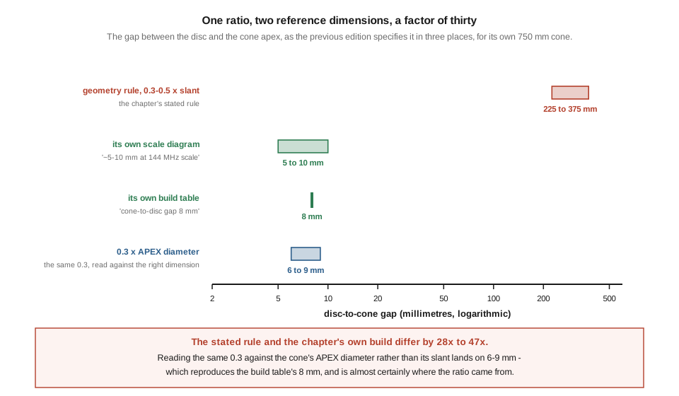
The chapter specifies the disc-to-cone gap in three places, and they do not agree.

In its geometry section, as a rule: “Gap distance (between disc and cone apex) = 0.3–0.5 × cone slant”.

In the scale diagram a few lines above it: ”← critical: ~5-10 mm at 144 MHz scale”.

In the DIY build’s dimension table, for a cone of 75 cm slant: “Cone-to-disc gap | 8 mm”.

🔴 The stated rule and the chapter’s own build differ by a factor of 28 to 47. Applied to the build’s own 750 mm cone, “0.3–0.5 × cone slant” demands a gap of 225 to 375 mm — a disc floating a third of a metre above the cone. The build table says 8 mm. The diagram says 5 to 10 mm. Two of the three statements agree with each other and with every discone ever photographed; one is out by a factor of thirty.

The reconstruction is straightforward and points at the same failure as §3. Read the 0.3 against the cone’s apex diameter rather than its slant and the numbers land:

Table 2 — 4. The feed gap, stated three times

apex diameter	0.3 × apex
20 mm	6.0 mm
25 mm	7.5 mm
30 mm	9.0 mm

⭐ That reproduces the build table’s 8 mm almost exactly, for the apex hardware size any real discone uses — the chapter’s own build specifies a hub of about 3 cm. So the ratio is probably right and its reference dimension has been swapped, exactly as in §3, and this time the swap is between two lengths differing by a factor of thirty rather than a factor of two. Same class of defect, thirty times the consequence.

⚠ What the gap actually does is worth stating, because it is the one dimension where the chapter’s instinct is sound. Its diagram calls the gap “critical”, and that is right. Vol 1 §3 counted the gap as one of the three lengths that disqualify a real discone from being frequency-independent, and it is the one that eventually spoils the match at the top of the band: while the gap is electrically tiny the feed behaves as a point, and when it stops being tiny the feed region becomes a transmission line of its own with its own behaviour. At 8 mm the gap is 0.0035 λ at 130 MHz and 0.035 λ at 1300 MHz — small throughout, which is why a well-built discone’s match survives to the top of its published range.

So the practical rule is a bound rather than a target: make the gap as small as the insulator and the working voltage allow. There is no benefit to a larger one and the chapter’s stated rule would ruin the antenna.

⚠ One thing is not settled here. The working voltage across that gap under transmit is the constraint on how small it can go, and no manufacturer among the five surveyed in Vol 5 publishes it. The chapter’s power-handling table lists “disc-cone gap dielectric | 100–500 W” with no gap dimension attached, which is an unusable specification. Computing the breakdown limit properly needs the feedpoint voltage at the design power, and that is a bench measurement rather than a literature one.

2.5 Solid, spoked, and the spoke count with no frequency in it

The chapter’s account of spoked construction is mostly good and contains one error of exactly the kind this dive keeps finding.

What it gets right, and this dive endorses: a spoked disc and a spoked cone are electrically equivalent to solid ones provided the spokes are close enough together in wavelengths; the motive is wind loading; and the failure mode at the high end is that the structure “starts to look like discrete radiators rather than a continuous cone”. All of that is correct, and §2 has now supplied the historical reason the wind mattered in the first place.

What it gets wrong is the criterion:

The number of spokes matters: at the high end of the discone’s frequency range, the spoke-to-spoke spacing approaches λ/4 and the antenna starts to look like discrete radiators rather than a continuous cone. 8 spokes are adequate for 1 GHz operation; 16 spokes give cleaner pattern at the high frequency end.

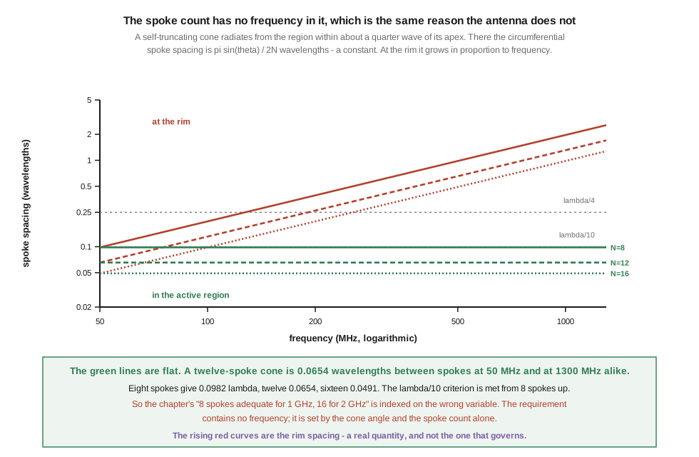
🔴 The requirement contains no frequency, and the reasoning that says it does uses the wrong part of the cone.

Here is the derivation. The spokes radiate from the apex, so their circumferential separation depends on how far down the cone you look. At a distance r from the apex, N spokes on a cone of half-angle θ are separated by

spacing = 2 π r sin θ / N

The chapter evaluates this at the rim, where r is the full slant height — a fixed length — so the spacing is a fixed length too, and measured in wavelengths it grows in direct proportion to frequency. That is the rising red curve in the figure, and it is a real quantity. On a 1.5 m cone at 30°, twelve spokes sit 0.393 m apart at the rim: 0.07 λ at 50 MHz, 0.59 λ at 450 MHz, and 1.70 λ at 1300 MHz. Read that way the chapter’s worry is well founded and its answer is far too optimistic — eight spokes would be 2.55 λ apart at 1300 MHz.

But the rim is not where the antenna is working. A conical antenna is self-truncating: at any frequency the radiating region is the part of the cone within roughly a quarter wave of the apex, which is precisely the mechanism Vol 1 §4 identified as the source of the constant characteristic impedance. The active region is not a fixed length. It scales with wavelength. So put r ≈ λ/4 into the spacing formula and the wavelength cancels:

spacing / λ = π sin θ / 2N

Table 3 — 5. Solid, spoked, and the spoke count with no frequency in it

spokes	spacing in the active region (θ = 30°)
4	0.1963 λ
6	0.1309 λ
8	0.0982 λ
12	0.0654 λ
16	0.0491 λ
24	0.0327 λ

⭐⭐⭐ There is no frequency in that table. A twelve-spoke cone is 0.0654 wavelengths between spokes at 50 MHz and at 1300 MHz and at 3 GHz. The antenna’s discretisation is frequency-independent for exactly the same reason its impedance is — both follow from the cone’s self-similarity, and the active region slides up the cone as the frequency rises, finding the spokes closer together in proportion.

Inverting the formula against the usual criteria:

Table 4 — Inverting the formula against the usual criteria

criterion	spokes required
spacing < λ/4	4
spacing < λ/10	8
spacing < λ/20	16

⭐⭐ That derives the published rules of thumb exactly. “Eight spokes minimum” is the λ/10 criterion; “sixteen for a cleaner job” is λ/20. The chapter arrives at the same two numbers and attaches them to frequencies — 8 for 1 GHz, 16 for 2 GHz — when they are not frequency thresholds at all. ⚠ The advice is therefore accidentally sound and the reason given for it is wrong, which is a distinction worth preserving: a builder following the chapter will choose the right spoke count, and a builder trying to extend an existing design to a higher band on the chapter’s reasoning will add spokes that buy nothing.

⚠ Two caveats belong with this. The self-truncation picture is a standard first-order model, not a measurement; the active region is a diffuse thing with no sharp edge, and treating it as “within λ/4 of the apex” is a convention. And the result says nothing about the disc, whose spokes radiate from a hub of fixed size over a fixed radius, so the disc’s discretisation genuinely does worsen with frequency in the way the chapter describes. The cone is frequency-independent in its spoke count; the disc is not. That asymmetry is not in the chapter and follows directly from which of the two structures is self-similar.

2.6 The dimensions nobody specifies

Three quantities govern a real build and appear in neither the chapter nor the published rules, and they are listed here because a builder meets all three in the first hour.

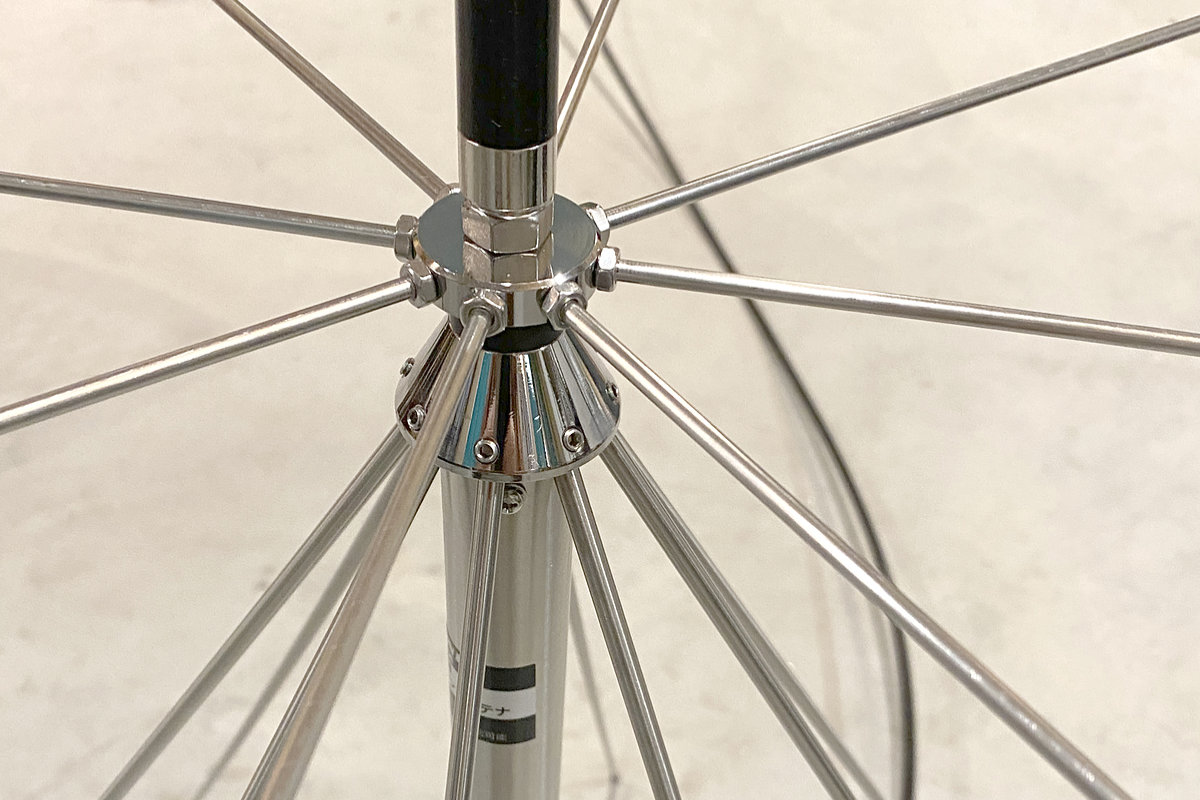
Spoke diameter. The cone is a conductor of revolution approximated by rods, and a rod’s effective width matters to the approximation in the same way a Yagi element’s diameter matters to its length. Nothing in the amateur literature surveyed here specifies it. The photographed antennas use rod of a few millimetres; the chapter’s build calls for 3/16″ welding rod, which is reasonable but unsupported.

Whether the cone’s rim is bonded. A ring joining the spoke tips makes the cone closer to a solid surface at the rim and adds wind loading and weight. The chapter says “The cone base is open (no perimeter ring needed — wind transparent)” for the cone while specifying a perimeter ring for the disc. ⭐ That asymmetry is defensible on §5’s argument — the cone’s rim is outside the active region at every frequency above the very bottom of the band, while the disc’s rim is always at its working radius — and it is worth recording as a case where the chapter’s practice is better than its stated reasoning.

The apex hardware’s size. §4 showed that the gap rule is almost certainly measured against this, and it is the one dimension on which the whole feed region depends. No source gives it.

⚠ These are recorded as gaps in the literature rather than as defects in the chapter. They are also exactly the sort of thing a single careful set of measurements on one commercial antenna would close, which is Vol 5’s standing theme.

2.7 Static, lightning and the DC path

The chapter offers two protective measures and the second is sound:

• DC short at the apex: a small ferrite bead with a short conductor across the apex provides a DC return path that drains static accumulation but is invisible at RF (the ferrite blocks RF current). Many commercial discones include this.
• Polyphaser arrestor at the bulkhead: blocks high-voltage transients before they enter the shack.

✅ The arrestor recommendation is correct and is carried forward unchanged. A gas-discharge or quarter-wave-stub arrestor at a single-point bulkhead ground is the standard of practice for any permanent outdoor installation, and it is the measure that actually protects equipment.

⚠ The DC-short description does not hold together as written, and the honest statement is that this dive could not establish commercial practice. The difficulty is the word “invisible”. A conductor bridging the feed gap has to present a high impedance across the entire operating range — 25 MHz to 1300 MHz on the antennas in Vol 1 §6, a 52:1 span — and a single ferrite bead does not do that. A bead’s impedance is a broad, lossy resonance of a few hundred ohms at best, which is not high against the antenna’s 50-odd ohms, and no bead holds a useful impedance over fifty-to-one. The devices that genuinely do this job are a large-value resistor, which drains static while being negligible in parallel with the feedpoint, or a quarter-wave shorted stub, which is a high impedance at one frequency and its odd multiples and therefore not wideband either.

⚠ Whether commercial discones include such a path at all could not be verified. None of the five manufacturers surveyed publishes a schematic of the feed region, and the claim that “many commercial discones include this” is repeated here as the chapter’s rather than endorsed. A builder should not assume a discone is DC-grounded, and should not assume it is not — it is a continuity check with a multimeter across the connector, taking ten seconds, and it is worth doing before connecting anything with a DC-coupled front end or a bias tee.

⭐ That last point is the one with practical teeth, and the chapter does not make it. A wideband SDR fed from a masthead preamplifier over a bias tee cares a great deal whether the antenna at the far end is a DC short. The active splitters dive covers the bias-tee side of that question.

2.8 Where this volume hands off

The geometry is now specified with its reference dimensions attached, which is the whole of what this volume was for.

The founding patent contains no dimensions, was assigned to a manufacturer rather than to a regulator, and was filed for an aircraft application whose wind-loading requirement is the ancestor of every spoked discone since. The disc is 0.7 of the cone’s slant, which is 0.7 of a quarter wave at the lowest frequency — and the disc-to-base form of the same rule is a different statement that happens to agree at 30°, the angle everyone builds at and the angle the previous edition’s own text specifies while its tables say 60°. The feed gap is a small fraction of the apex diameter and comes out at millimetres; the chapter’s “0.3–0.5 × cone slant” is the same ratio read against a length thirty times too large, and its own build table has it right. And the spoke count is set by π sin θ / 2N with no frequency in it, which derives the familiar eight-and-sixteen rules from the λ/10 and λ/20 criteria and shows that the chapter’s frequency thresholds are not thresholds.

From here:

• Vol 3 — The pattern is where this dive expects its largest correction. The chapter states that a discone peaks at 25–35° of elevation and is weak toward the horizon; the published accounts say its sensitivity is highest at the horizon. Vol 1 §7 left the top-of-band behaviour as a bound; Vol 3 computes it.
• Vol 4 — The rest of the family takes the symmetric biconical, the conical monopole, the sleeve and the bow-tie, and the EMC-test instruments where a biconical is a calibrated object rather than a scanner accessory.
• Vol 5 — Build, measure and buy builds the antenna this volume has just re-specified, with the angle corrected and the gap rule replaced, and surveys the market with a date on it.

Two things are owed. The primary source of the dimensional rules, which §2 could not trace past two secondary works. And the three unspecified dimensions in §6, every one of which a morning with a commercial antenna and a pair of calipers would settle.

2.9 Resources

• Armig G. Kandoian, Broad band antenna, US Patent 2,368,663 — filed 15 May 1943, granted 6 February 1945, assigned to the Federal Telephone and Radio Corporation. Read in full for §2. The primary source, and notable for what it does not contain.
• Jerry Hall, ed., The ARRL Antenna Book, 16th ed., 1991, pp. 7–17 — one of the two secondary works carrying the disc and cone-angle rules §3 examines.
• Paul Lee, The Amateur Radio Vertical Antenna Handbook, 2nd ed., CQ Communications, 1996, pp. 50–51 — the other.
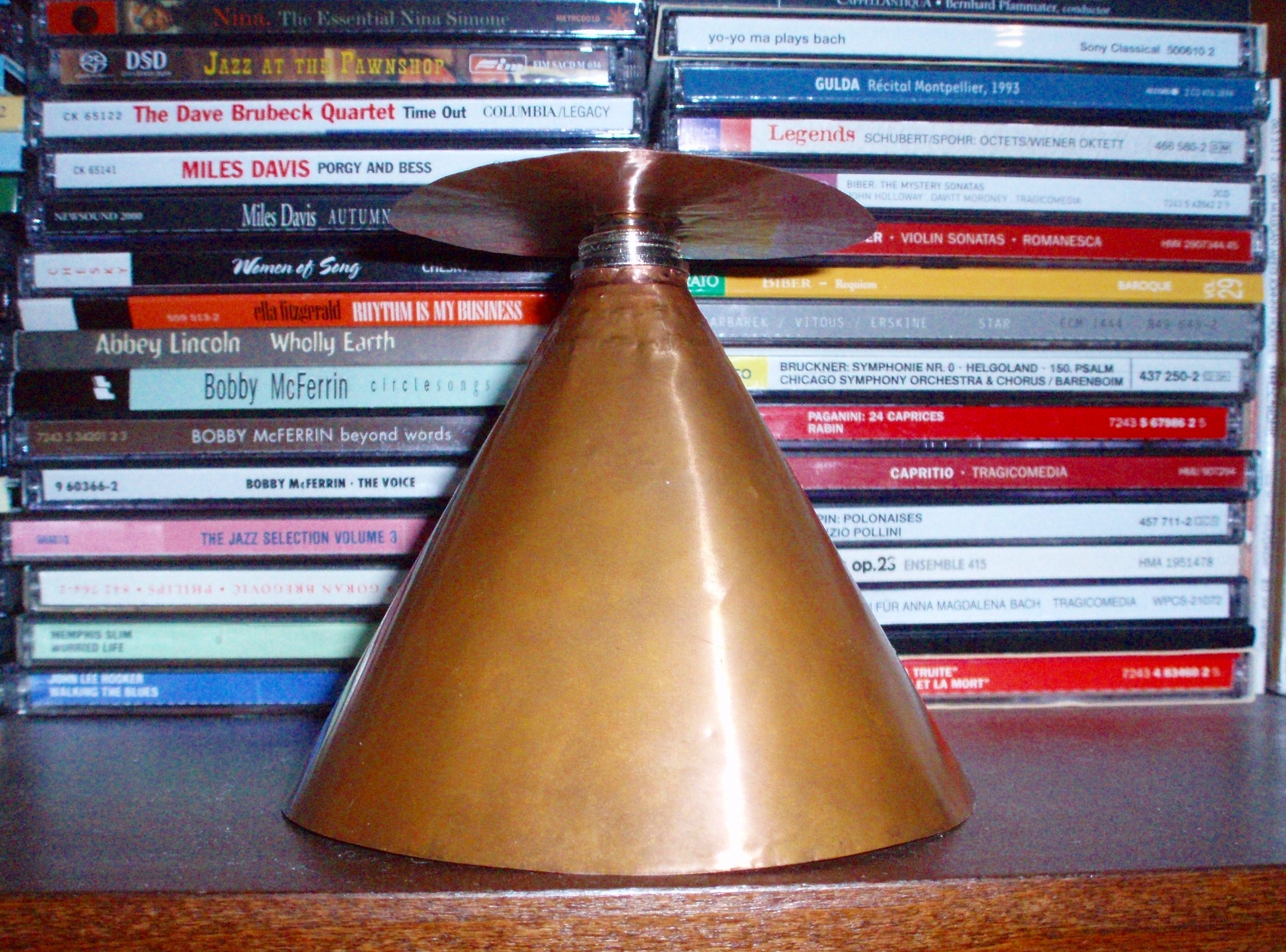
• Wikimedia Commons, Discone-solid-copper-700Mhz-2Ghz.jpg, by Adamantios, CC BY-SA 3.0 — the antenna measured in Vol 1 §4 and the lead image here.
• Discone and wideband antennas, Vol 1 — the cone angle that sets the impedance, and the factor-of-two error that propagates into every ratio in this volume.
• Yagi-Uda antennas, Vol 3 — element diameter as a correction to element length, the closest analogue to §6’s unspecified spoke diameter.
• Active splitters and preamps, Vol 1 — bias tees and masthead preamplifiers, and why §7’s DC continuity check matters before one is connected.
• Log-periodic and structured wideband antennas — the other way of building a wideband antenna, where the discretisation §5 treats as an approximation becomes the operating principle instead.