Non-Resonant Wires — Random, Long, Inverted-L and Sloper

---

3.1 About this volume

Vol 2 built an antenna around resonance: cut the wire to a half-wave, accept the harmonic series that follows, and let a fixed-ratio transformer meet a feedpoint impedance you have arranged to be predictable. This volume takes the opposite design philosophy. Put up whatever length of wire the lot allows, accept that its feedpoint impedance will be different on every band and inconvenient on most of them, and hand the problem to a tuner.

That is not a cheaper version of the same antenna. It is a different bargain, with different failure modes, and it is worth being clear about which one you are making. The resonant end-fed half-wave buys a clean match on a few bands at the cost of being cut for one specific band plan. The random wire buys continuous coverage of everything from 160 m up at the cost of never presenting a clean match anywhere, needing a matching network in the shack, and — the part this volume spends most of its time on — being unexpectedly sensitive to a length that was supposed to be arbitrary.

Four things drove the sections below, and three of them are corrections.

“Random” is a misnomer, and the seed’s own recommended lengths prove it. §2 derives the feedpoint resistance of a wire fed at its end as a function of frequency, and §3 audits all six lengths the previous edition recommended against every HF band. Four of the six land on an exact or near-exact half-wave multiple somewhere inside an amateur band, and the one length the chapter flagged as risky was flagged for the wrong band — it is far worse on 40 m and 10 m than on the 20 m it warned about. The section replaces the folklore table with a derived rule and a number.

A 9:1 transformer does not compress an impedance range. The previous edition said that without it a tuner sees 20 Ω to 5000 Ω, and with it “the range compresses to ~5 Ω to 500 Ω.” §4 shows that dividing every impedance by nine leaves the ratio of largest to smallest exactly where it was — 250:1 before and 250:1 after. The transformer re-centres the range on 50 Ω, which is genuinely useful and is the real justification, but it cannot narrow it, and on a band where the wire already looked low it makes the match distinctly worse.

The long-wire lobe table is right up to two wavelengths and drifts badly after that. §6 computes the patterns rather than redrawing them. At 1λ, 1.5λ and 2λ the previous edition’s angles are correct to within a degree. At 4λ, 8λ and 16λ they understate the lobe angle by 2°, 3.6° and 5.4° respectively, which makes the antenna sound more sharply end-fire than it is.

And one thing the seed got right, which a number makes better. §8’s claim that an inverted-L’s short vertical section is what does the low-angle radiating is correct, and it becomes much more persuasive once you compute the current distribution: on a 160 m inverted-L with a 30 ft vertical and 100 ft of horizontal top wire, the vertical carries 44 % of the total current-squared on 23 % of the wire.

3.2 What “random” actually means

A wire fed at one end with its far end open carries a standing wave fixed by that open end: the current must be zero there. Writing z for distance from the feedpoint and L for the wire’s length,

I(z) = I₀ · sin(β(L − z))

so at the feedpoint itself, I(0)/I₀ = sin(βL) = sin(πm), where m = L / (λ/2) is simply the wire’s length measured in half-waves at whatever frequency you are using. Vol 1’s argument then gives the resistance directly: radiated power is a property of the whole antenna, so the resistance at the feed must rise as fast as the current there falls,

R = R_ref / sin²(πm)

with R_ref the resistance at a current maximum, taken as 73 Ω. That simplification ignores the slow rise of radiation resistance with wire length and the mutual coupling between half-wave sections, so the absolute values below are indicative rather than exact — but the shape, which is what the section is about, is right.

Read the formula and the whole random-wire design problem falls out of it:

• When m is a half-integer — the wire is an odd number of quarter-waves — sin(πm) = ±1 and R = 73 Ω. This is the friendly case, and it needs no transformer at all.
• When m is an integer — the wire is a whole number of half-waves — sin(πm) = 0 and R → ∞. This is the case Vol 2 built an antenna out of deliberately, with a 49:1 transformer to meet it. On a random wire it is a disaster, because there is no fixed ratio waiting for it.
• Everywhere in between, R sweeps between those extremes, and it does so fast near the integers.

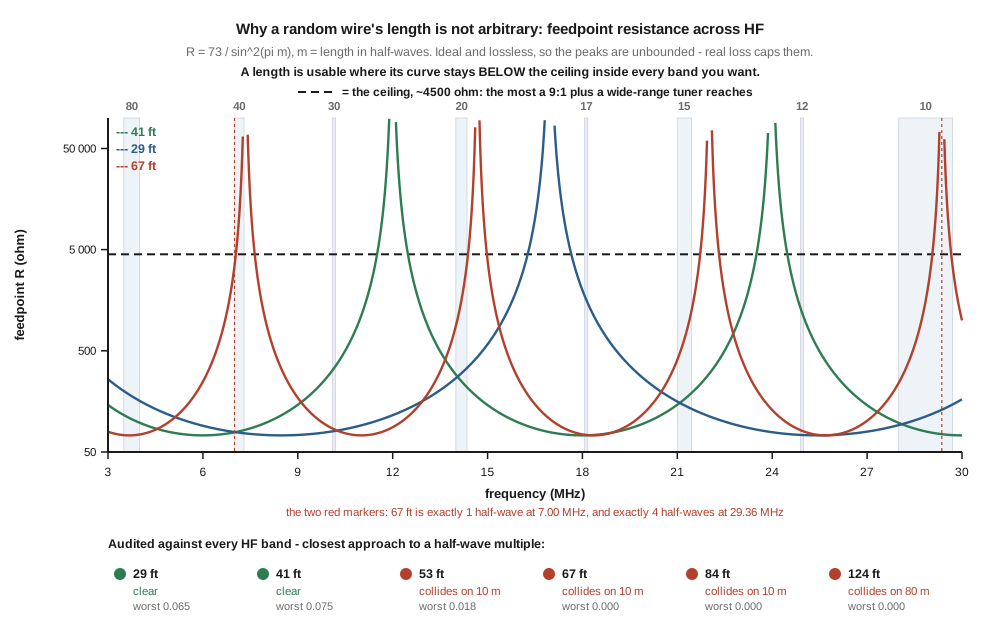
The lead figure plots this across HF for three lengths. The peaks run off the top of the chart because the ideal model is unbounded, exactly as at the tip of a half-wave in Vol 1; real loss caps them at some finite but still very large number. What matters is not the height of the peaks but where they fall relative to the bands you want to use.

So “random wire” means a wire whose length was not chosen for resonance. It does not mean a wire whose length does not matter. Those are very different claims, and the second one is false.

3.3 Auditing the recommended lengths

The previous edition offered six lengths as reliable across 80–10 m. Each has been checked here against every US HF amateur allocation, at 400 points across each band, for the closest approach to an integer number of half-waves.

First, the threshold — because “avoid half-wave multiples” is useless without a number attached. Take a wide-range tuner that will match up to about 10:1 at its input, so up to roughly 500 Ω, sitting behind a 9:1 transformer. That puts the ceiling on the antenna-side resistance at about 4500 Ω. Inverting the formula in §2:

sin(πδ) ≥ √(73 / 4500) = 0.127 ⟹ δ ≥ 0.041

The feedpoint must stay at least about 4 % of a half-wave away from every integer multiple, in every band you intend to use. That is the rule the folklore table is groping toward, and unlike the table it can be checked.

Table 1 — 3. Auditing the recommended lengths

Length	Closest approach	Where	Verdict
29 ft	0.065	17 m	clear
41 ft	0.075	12 m	clear — and the best of the six
53 ft	0.018	bottom edge of 10 m	collides
67 ft	0.005	7.00 MHz	collides badly
84 ft	0.000	29.28 MHz	collides exactly
124 ft	0.000	3.97 MHz	collides exactly

Three things are worth drawing out of that table, and the first is a correction to my own instinct rather than to the seed.

The seed’s headline claim is right: 41 ft is the good one. Its worst approach anywhere in HF is 0.075 — nearly twice the threshold, and it occurs on 12 m, the narrowest and least-used band in the list. At that worst point the model gives about 1340 Ω, which through a 9:1 is 149 Ω, about 3:1 at the tuner. Comfortable. The reputation is earned, and an early version of this audit that used a tighter threshold flagged 41 ft as problematic — which was the threshold’s fault, not the wire’s. A scary-looking proximity number is not a defect until you attach a tuner to it.

Four of the six collide, and the chapter flagged only one of them — for the wrong band. The previous edition’s single caution was that 67 ft “edges close to 1λ at 14 MHz.” It does: 1.91 to 1.96 half-waves across 20 m, a closest approach of 0.045, which is just inside the threshold and genuinely marginal. But 67 ft is exactly one half-wave at 7.000 MHz — the very bottom of 40 m, in the middle of the CW segment — and exactly four half-waves at 29.36 MHz. Both are an order of magnitude worse than the case it warned about. Meanwhile 84 ft is exactly five half-waves at 29.28 MHz and 124 ft exactly one half-wave at 3.97 MHz, and neither carries any warning at all.

But the collisions are spots, not bands, and that is the genuinely useful finding. A wire does not become unusable on 10 m because it hits five half-waves at 29.28 MHz; it becomes unusable near 29.28 MHz. Move down to 28.3 MHz and 84 ft is 4.83 half-waves — 0.17 from an integer, comfortably clear. The same is true of 124 ft, whose 80 m problem sits at the top of the band while 3.6 MHz is fine, and of 67 ft, whose 40 m problem is at the CW edge while the phone segment is workable.

That reframes the advice usefully. The question is not “is this length good?” but “where are this length’s bad spots, and do I care about those frequencies?” A 124 ft wire is an excellent 80 m antenna for someone who lives at the bottom of the band and a poor one for someone who operates 3.95 MHz nets. The old table cannot express that; the formula can, and the calculation is a few lines of arithmetic per length.

One caution against over-reading this section. Real wires are not the ideal model: loss caps the peaks, the counterpoise and feedline are part of the system, and a tuner’s real match range depends on its topology and on the reactance it is fighting as much as on the resistance. A length that the model says collides may still tune, unhappily and with loss in the tuner. The audit identifies where to expect trouble, not where operation is impossible. Several popular “magic length” tables circulate that were not verifiable for this volume; the honest advice is to run any candidate through the arithmetic above against the bands you personally use, rather than to trust a list — including this one.

3.4 The 9:1 and what it actually does

A 9:1 unun presents 9 × 50 = 450 Ω on its antenna side when the rig sees 50 Ω. The previous edition explained its purpose like this:

Without the 9:1, the tuner sees impedances ranging from 20 Ω to 5000 Ω across the bands — beyond most tuners’ match range. With the 9:1, the range compresses to ~5 Ω to 500 Ω, which any tuner handles.

The arithmetic does not support that. Dividing 20 Ω and 5000 Ω by nine gives 2.2 Ω and 556 Ω — not 5 and 500 — and more importantly:

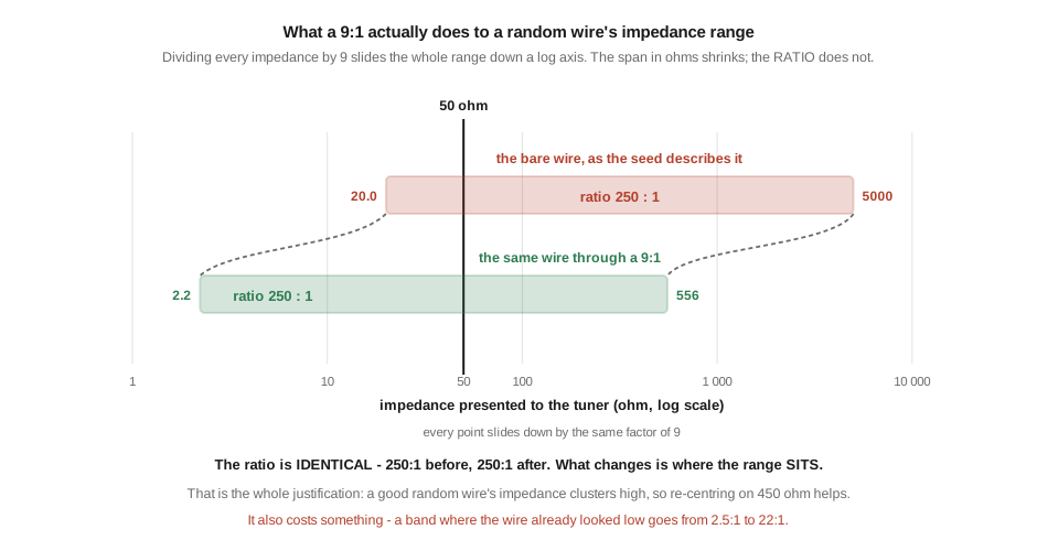
5000 / 20 = 250, and 556 / 2.2 = 250. The ratio is invariant. A fixed-ratio transformer is a multiplication, and multiplying every number in a range by the same constant slides the range along a logarithmic axis without changing its width. The span measured in ohms shrinks, which is presumably where the word “compresses” came from, but the span in ohms is not what determines whether a tuner can cope — the ratio to 50 Ω is.

Work that consequence through and the transformer’s real cost appears:

Table 2 — Work that consequence through and the transformer's real cost appears

	high end (5000 Ω)	low end (20 Ω)
bare wire, against 50 Ω	100:1	2.5:1
through a 9:1	11:1	22:1

The high end improves by ninefold, which is the whole point. The low end gets nine times worse — a band where the wire happened to present a friendly 20 Ω, which a tuner would barely have noticed, becomes a 22:1 problem. Nothing was compressed. The distribution was slid nine steps down the axis, and whatever was already below 50 Ω went with it.

So why use one at all? Because a well-chosen random wire’s impedance is not uniformly distributed — it clusters high. §2’s formula spends most of its range above R_ref, since sin²(πm) ≤ 1 always, and a length audited by §3 to stay clear of the integers still spends most of HF in the hundreds to low thousands of ohms. Re-centring that cluster on 450 Ω puts far more of it near 50 Ω than leaving it alone would. The 9:1 is a bet that the wire’s impedance is high, and §3’s length rule is what makes the bet a good one. They are not two independent design choices; they are the same choice, and a builder who ignores the length rule has also undermined the transformer.

The honest summary is that a 9:1 shifts the problem into the range where a tuner is effective, and that “any tuner handles it” is too strong — §5.

3.4.1 The core, and one row that does not survive checking

The previous edition’s core table listed an iron-powder option:

T200-2 · iron powder (red) · RX-only · 1–60 MHz — very low loss but core saturation under sub-100 W transmit.

The disqualification is real; the stated reason is not. Iron-powder mix 2 has an initial permeability of about 10, against roughly 800 for ferrite mix 43, and the consequence is easy to compute. A T200-2 has an A_L of about 120 µH per 100 turns, so a 9-turn winding gives

L = 120 × (9/100)² = 0.97 µH

and at 3.5 MHz that is a magnetising reactance of 21 Ω. The design rule quoted in Vol 1 from VK3IL — that you want at least 200 Ω on the transformer’s primary so the transformer does not dominate what the transmitter sees — is missed by a factor of ten. The same 9 turns on an FT240-43 gives about 87 µH, which at 3.5 MHz is on the order of a thousand ohms or more. ⚠ That ferrite figure uses the low-frequency A_L, and mix 43’s permeability is already falling by 3.5 MHz, so the true reactance is lower than the naive calculation gives; iron-powder mix 2, by contrast, holds its permeability flat well past 30 MHz, which is its one genuine virtue. The comparison survives the correction comfortably — the gap is one to two orders of magnitude, and no permeability roll-off of that size exists. The iron-powder core fails as a broadband HF transformer because it cannot develop enough magnetising inductance, not because it saturates.

That distinction matters beyond this one table row, because it is the third instance in this dive and its companion of an inductive or thermal limit being described as saturation. The seed’s own power section carries the same misframing — the failure mode there is thermal, and the correction belongs to Vol 5 — and so does the BALUNs and UNUNs dive, where the finding is stated in full: saturation is usually the wrong worry. Where iron powder genuinely does fail in HF service it fails by overheating, which is a different symptom with a different remedy.

The broader ferrite-mix question — 43 against 31 against 52, and which is resistive where — is not re-derived here. It belongs to BALUNs and UNUNs Vol 3, which treats it at transformer-designer depth, and the winding procedure for a trifilar 9:1 belongs to Vol 5 of that dive. ⚠ One flag rather than a correction: the previous edition justified mix 43 on the grounds that its loss damps resonances and flattens the response. Loss is not usually a property you want in a transmitting transformer, and the loss measurements collected for Vol 4 of this dive make that trade explicit. The core prices the old table quoted have been dropped rather than repeated — they were unattributed, and this program has previously shipped fabricated “verified” prices.

3.5 Why the tuner is not optional

A random wire plus a 9:1 does not present a clean match on any band. That is not a defect in the installation; it is the design. The transformer’s job was to move the impedance into a range a tuner can work with, and the tuner’s job is everything after that.

Two practical consequences follow.

The tuner must be a real one, and where it sits matters. Modern transceivers with internal tuners — the IC-7300 and FT-991A being the common examples — are generally specified to about 3:1, which is a matching range chosen for trimming out a resonant antenna’s band-edge behaviour rather than for absorbing a random wire. §4’s table shows a 9:1-fed random wire reaching 11:1 at the high end and worse at the low end, well outside that. A wide-range external tuner is the right tool. It is also worth remembering that a tuner in the shack does not improve the antenna — it presents the transmitter with a load it will run into, while the mismatch, and the loss it drives, remain on the feedline between the tuner and the wire. Tuning at the antenna feedpoint rather than at the rig avoids that, and the antenna tuners dive covers the trade in full.

Receive is a different problem, and a much easier one. For a receive-only installation — an SDR listening across HF, a shortwave receiver, a scanner — the tuner is unnecessary. A software-defined receiver tolerates a poor match happily, because at receive the mismatch costs signal and noise in the same proportion, and on HF the external noise floor rather than the receiver’s own noise figure sets what you can hear. A few decibels of mismatch loss ahead of an already noise-dominated band changes very little. That is why a random wire, a cheap 9:1 and a run of coax is such a durable recommendation for an SDR: it is the case where all of this volume’s compromises stop mattering.

⚠ The previous edition’s specific tuner model recommendations have not been re-verified against current catalogues and are not repeated here. Product lines move, and Vol 5 carries the dated commercial survey for this dive.

3.6 Long wires and where their lobes really point

A long wire is a wire that is several wavelengths long at the operating frequency, fed at one end. It is the same structure as everything else in this dive; what changes is that once the wire is more than about two wavelengths long its pattern stops resembling a dipole’s and starts resembling a searchlight.

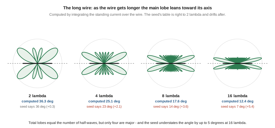
The patterns above were computed by integrating the standing current distribution over the wire, the same method Vol 2 used for the harmonic bands. Against the previous edition’s table:

Table 3 — The patterns above were computed by integrating the standing current distribution over the wire, the same method [Vol 2](/random-wire-end-fed/vol-2/) used for the harmonic bands. Against the previous edition's table

Wire length	Seed’s angle	Computed	Difference
1 λ	54°	53.9°	−0.1°
1.5 λ	42°	42.6°	+0.6°
2 λ	36°	36.3°	+0.3°
4 λ	23°	25.1°	+2.1°
8 λ	14°	17.6°	+3.6°
16 λ	7°	12.4°	+5.4°

The table is accurate to two wavelengths and then drifts, always in the same direction: it understates the angle, making the antenna sound more end-fire than it is. The divergence is not a rounding artefact — by 16λ the claimed 7° is nearly half the computed 12.4°. The computed values can be checked against the standard closed-form approximation for a resonant long wire, cos θ = 1 − 0.371 λ/L, and the two methods agree to within 0.2° from four wavelengths up — which is worth noting, because it is exactly the region where the old table goes wrong, and two independent methods agreeing there is better evidence than either alone. ⚠ The closed form is a poorer approximation at short lengths, diverging from the integrated pattern by 0.8° at 2λ and by nearly 3° at 1λ, and applied to a half-wave it returns 75° for an antenna that is unambiguously broadside at 90°. Use it above a couple of wavelengths and not below.

The lobe counts in the old table survive. The total number of lobes on one side of the wire equals the number of half-waves — eight for a 4λ wire, thirty-two for a 16λ one — but only four in the full plane are major, the rest falling away steeply. Describing a long wire as a four-lobe antenna is a fair simplification.

What all of this is for, practically:

• The gain is real but it is not steerable. A long wire’s main lobes point at a fixed pair of angles either side of the wire’s axis, set by its length in wavelengths — which means they point somewhere different on every band. Changing the favoured direction means moving the wire.
• Very long wires approach the rhombic. Past about eight wavelengths the pattern is strongly end-fire, and the classical terminated rhombic — four such wires in a diamond, terminated at the far apex to make the current travelling rather than standing — is the logical conclusion of the idea. That was the workhorse of long-haul HF broadcasting and point-to-point services through the middle of the twentieth century, and it needs acreage.
• The modern niche is receive. A long wire’s directivity is as useful for rejecting noise and off-path interference as for gain, and it costs nothing to feed it into a receiver. The terminated Beverage — a long, low, terminated receive wire — is the specialised form, and it belongs to the receive-only loops dive rather than here.

⚠ The previous edition claimed 3–6 dB of directional gain for a long wire over an end-fed half-wave. That is a plausible figure for a wire of several wavelengths in its favoured direction, but no source was found for it and it is not reproduced as a specification. What can be said from the computed patterns is the shape of the claim: the gain is concentrated into four narrow lobes, it grows with length, and it is paid for in every other direction.

3.7 The end-fed long wire

Between the resonant half-wave of Vol 2 and the multi-wavelength long wire of §6 sits a design the previous edition calls the end-fed long wire: a wire deliberately cut longer than a half-wave — a full wavelength at the lowest band, say — and fed through a higher-ratio transformer.

The mechanical argument for it is sound. A 1λ wire is two half-waves collinear with each other, so on its design band it has modestly more gain than a half-wave and a narrower main lobe, and it retains a high feedpoint impedance for the same reason a half-wave does: the end is still a current null. The distinction between “EFHW” and “EFLW” is convention rather than physics, and the previous edition says so, which is right.

⚠ One number in that section should not be repeated without a flag. The chapter states that the feedpoint impedance of a full-wave end-fed is “~4000 Ω” and that a 64:1 or 81:1 unun is therefore correct. Note that 81 × 50 = 4050. This is the third target impedance in this dive to equal its transformer ratio times fifty — the 2450 Ω and 3200 Ω cases were both traced to exactly that circularity and corrected in earlier passes. Whether this figure was arrived at the same way cannot be established from the source, and 4000 Ω is also quoted independently in the amateur literature as a rough empirical figure for full-wave end-feds, so it is not being declared wrong here. What can be said with confidence is Vol 1’s conclusion: the end impedance of an integer-half-wave wire is unbounded in the ideal model and finite only because of loss and loading, so no formula produces 4000 Ω, and any specific figure is a statement about a particular installation. Choose the ratio against a measured impedance — the procedure is in Vol 4 — rather than against a table.

The practical position is that an end-fed wire longer than a half-wave is a reasonable thing to build if the space exists, that it wants its transformer selected by measurement, and that as it grows past two wavelengths it stops being a general-purpose antenna and becomes the directional one §6 describes.

3.8 Slopers and inverted-Ls

The last two variants are geometric rather than electrical: the same end-fed wire, hung in a shape that does something useful.

3.8.1 The sloper

A sloper is a wire — resonant or not — with one end high and the other low, typically fed at the top from a tower or mast and descending at 30° to 60°. It is popular on the low bands, where a full-size horizontal antenna at a useful height is not a realistic proposition on a residential lot.

The previous edition described its polarisation like this: “vertical polarization in the lower half of the antenna (~50%), horizontal polarization in the upper half (~50%).” That is not how a sloping wire works. Polarisation is set by the direction of the current, and the current on a straight wire runs along the wire everywhere on it. A wire at 45° has equal vertical and horizontal current components along its entire length, not vertical components at the bottom and horizontal ones at the top. The mix is set by the slope angle: a steeply hung wire is mostly vertically polarised over all of itself, a shallow one mostly horizontally polarised over all of itself, and a 45° wire is an even mix everywhere.

The conclusion the old text drew from its wrong premise happens to be right, which is worth saying plainly rather than throwing out with the explanation. A sloper does radiate a mix of polarisations, and it is directionally biased toward the low end. The reason for the bias is not the polarisation split, though — it is that a top-fed sloper off a grounded metal tower is a two-element system in which the tower carries current and acts as a parasitic element. That is also why slopers off a tower behave differently from slopers off a fibreglass mast, a distinction the geometry-only account cannot make.

⚠ The 2–5 dB figure the previous edition gave for the front-to-back bias is unattributed and is not reproduced as a specification. Reported figures for tower-mounted slopers vary widely with tower height, guy arrangement and what else is mounted on the tower, which is consistent with the tower being the second element.

3.8.2 The inverted-L

An inverted-L is a vertical section with a horizontal top section, fed at the base against radials. It is the standard answer to 160 m and 80 m on a small lot, and it is the one antenna in this volume where the seed’s reasoning is correct and only needed a number.

The claim was that the vertical section provides the low-angle radiation without needing a full-size vertical’s height. Take the worked example: 30 ft of vertical, 100 ft of horizontal top wire, 130 ft in total, at 1.9 MHz where a quarter wave is 129.4 ft. The wire is therefore 100.5 % of a quarter wave — the arithmetic checks — and being base-fed and roughly a quarter wave, the current maximum is at the feedpoint, at the bottom of the vertical.

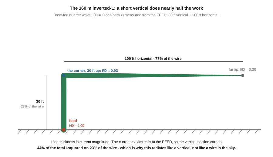
Computing I(z) = I₀ cos(βz) along the wire from the feed gives the current at the corner, 30 ft up, as 0.93 of the maximum, falling to zero at the far tip. Integrating the square of the current — which is what the radiating contribution scales with — over each section:

The 30 ft vertical carries 44 % of the total, on 23 % of the wire’s length.

That is the whole antenna in one number. Nearly half the radiating work happens in the vertical section, at the low elevation angles a vertical produces, while the horizontal top wire’s job is largely to bring the structure to resonance in a space that has no room for another hundred feet of height. It is not a horizontal antenna with a feed dropped to the ground; it is a short vertical with a capacity hat made of wire.

Three consequences follow, and they are the reasons this antenna is more work than it looks:

• The radial field is not optional. The current maximum is at the feedpoint, at ground level, and that current has to return through the ground system. A quarter-wave vertical with a poor ground turns a large fraction of its input into heat in the soil. This is the one antenna in this dive that genuinely needs radials rather than a counterpoise, and it is the exception to Vol 1’s argument about end-fed antennas not needing a ground system — because it is not being fed at a voltage maximum. The fixed vertical monopole dive covers radial-field design properly.
• It is single-band by construction. Nothing about the geometry produces a usable harmonic series the way Vol 2’s end-fed does, and the resonance is set by the total wire length against a ground system.
• The horizontal section radiates too, mostly upward. The 56 % of the current-squared it carries is horizontally polarised at a low height in wavelengths — on 160 m, 30 ft is about 0.06 λ — which by Vol 2’s height argument is a near-vertical-incidence radiator. An inverted-L is therefore genuinely a hybrid: low-angle vertical for DX, high-angle horizontal for local work, in one structure.

3.9 Where this volume hands off

The non-resonant half of the family is now specified. A random wire’s length is not arbitrary: the feedpoint resistance follows 73/sin²(πm), it runs away near every integer number of half-waves, and a usable length is one that stays about 4 % of a half-wave clear of those integers in every band you actually use — a test that four of the six traditionally recommended lengths fail somewhere. A 9:1 transformer re-centres that impedance distribution on 50 Ω without narrowing it, which is worth doing because the distribution clusters high, and which costs real margin on any band where the wire looked low. A tuner is part of the antenna, not an accessory to it, except on receive where none of this matters much. A long wire’s lobes lean toward its axis as it lengthens, by angles that the traditional table gets right to two wavelengths and understates thereafter. And the two geometric variants both work by putting current where it does the most good — which in the inverted-L’s case is 44 % of it in the shortest 23 % of the wire.

From here:

• Vol 4 — Feed, counterpoise and the ground question is where every impedance in this volume stops being modelled and starts being measured: selecting a transformer ratio against a real feedpoint, the transformer loss that flatters an SWR reading, counterpoise length in the field, and common-mode current as the second device in the system. §7’s flagged 4000 Ω figure is settled there, by measurement rather than by table.
• Vol 5 — DIY build, measurement and buys builds and trims a wire with a VNA, and carries the dated commercial survey this volume deliberately does not.
• Vol 1 and Vol 2 hold the foundations this volume assumed: the standing-wave picture and the resistance derivation in Vol 1, and the harmonic series, the height argument and the fixed-ratio-into-a-variable-load problem in Vol 2.

Three items are owed against this volume. §3’s threshold assumes a tuner that reaches 10:1 at its input, which is a reasonable figure for a wide-range external unit but is an assumption, not a measurement — a reader with a different tuner should recompute the 4 % figure for it, and the arithmetic is in the section. §6’s gain claim and §8’s front-to-back figure are both unsourced and are flagged in place rather than repeated as specifications. And the figures here were generated numerically and checked against their formulas and by an XML bounds pass, but not rendered by a browser at authoring time, so they remain on the pre-publish check list along with Vols 1 and 2.

3.10 Resources

• Vol 1 — Why end-feeding works at all — the standing-wave derivation this volume’s §2 formula is the general case of, and the VK3IL 200 Ω primary rule used in §4.
• Vol 2 — The resonant end-fed half-wave — the resonant design this volume is the counterpart to, including the pattern-integration method reused in §6 and the height argument applied in §8.
• BALUNs and UNUNs, Vol 3 — complex permeability, the ferrite mix question, and the finding that saturation is usually the wrong worry, which §4’s iron-powder correction is the third instance of.
• BALUNs and UNUNs, Vol 5 — the trifilar winding procedure for a 9:1, which this volume deliberately does not duplicate.
• Antenna tuners, Vol 1 — matching-network topologies and the tune-at-the-rig versus tune-at-the-antenna trade referenced in §5.
• Fixed vertical monopoles, Vol 2 — radial-field design, which §8’s inverted-L genuinely requires.
• Receive-only loops, Vol 1 — the Beverage and the other terminated receive wires §6 hands off to.
• Amidon and Micrometals iron-powder core data — the A_L figure for the T200-2 used in §4’s computation. Iron-powder and ferrite data are not interchangeable and are frequently confused in amateur sources.