Random Wire & End-Fed Antennas · Volume 2
The Resonant End-Fed Half-Wave
Cutting the wire, why every harmonic works and not just the odd ones, which bands actually land and which are quietly missed, and what height and surroundings do to all of it
2.1 About this volume
Vol 1 established that a resonant wire carries a fixed current distribution, that feeding it at a voltage maximum rather than a current maximum changes the impedance and nothing else about the radiation, and that the impedance you find at the end is high, unbounded in the ideal case, and set in practice by loss and loading rather than by any constant. This volume takes that foundation and builds the antenna that made the family famous: the resonant end-fed half-wave, cut to a specific length and worked on several bands at once.
The multi-band behaviour is the whole commercial proposition. One wire, one transformer, one feedline, and four bands without a tuner — that is what an EFHW is sold as, and unlike a great many antenna claims it is substantially true. What is not true is most of the explanation that accompanies it, and this is a volume where the received wisdom and the arithmetic part company more than once.
Three corrections drive the sections that follow, and each is a case of a claim that has been repeated until it sounds like physics.
The first is that the end-fed half-wave works on “odd harmonics.” It does not; it works on every integer harmonic, odd and even alike, and the previous edition of this chapter contained a table that disproved its own claim two paragraphs after making it. §3 shows why the end of a wire is a current null for every integer multiple of a half-wave, and identifies where the odd-harmonic idea comes from — it is a centre-fed fact, imported into an end-fed context where it does not apply.
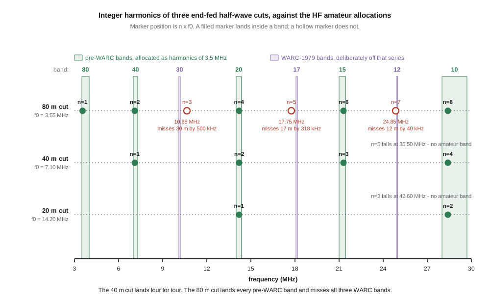
The second is that an 80 m end-fed half-wave covers the WARC bands. The integer harmonics of an 80 m wire miss 30 m by 500 kHz, 17 m by 318 kHz and 12 m by 40 kHz. §4 computes the whole series against the band edges and explains why the misses are structural rather than accidental: the traditional bands are harmonically related because they were allocated that way, and the 1979 WARC bands were deliberately placed off that series. This is also the section where over-correcting would be easy and wrong — vendors do sell 80 m end-feds advertised as covering 30, 17 and 12 m, and reviewers on those vendors’ own pages report needing a tuner to do it. The gap between the model and the product is the interesting part.
The third is that 6 m is the fifth harmonic of a 40 m end-fed. Five times 7.10 MHz is 35.50 MHz, which is not an amateur band in any region. The 6 m band sits at harmonic number 7.04 of a 40 m cut, and the seventh harmonic still misses the band edge by 300 kHz.
Everything in this volume that can be computed has been. The harmonic tables come from arithmetic against the ARRL band plan; the radiation patterns come from integrating the current distribution rather than from redrawing a textbook figure; the elevation angles come from the ground-reflection formula. Where a number could not be sourced or derived — the typical SWR values in §6 are the main case — it is presented as representative and labelled as such rather than dressed up.
2.2 Cutting the wire
The starting length is the free-space half-wave. With frequency in megahertz,
λ/2 = 149.90 / f metres = 491.8 / f feet
and no real antenna is that long, because the electrical length of a wire exceeds its physical length. The tips of the wire have capacitance to their surroundings, and that capacitance carries a little displacement current past the physical end of the conductor, so the standing wave behaves as though the wire continued a short distance into free space. The effect is called end effect, and its size depends on the wire’s diameter relative to its length, on insulation, and on what is near the ends.
The traditional amateur allowance is about five percent, which gives the constant every antenna book prints:
L ≈ 468 / f feet
That is 468 / 491.8 = 0.951, a 4.9 % shortening. Applied to the three common cuts:
Table 1 — That is 468 / 491.8 = 0.951, a 4.9 % shortening. Applied to the three common cuts
| Cut | f₀ | Free-space λ/2 | 468/f starting length | Bands claimed |
|---|---|---|---|---|
| 20 m | 14.20 MHz | 34.6 ft | 33.0 ft | 20, 10 |
| 40 m | 7.10 MHz | 69.3 ft | 65.9 ft | 40, 20, 15, 10 |
| 80 m | 3.55 MHz | 138.5 ft | 131.8 ft | 80 and up |
Those land on the lengths the market actually sells — the ARRL’s own end-fed kit is about 66 ft for 40/20/15/10 m, and the 80 m units cluster around 130 ft.
The 468 constant is a starting point for trimming, not a specification, and it is worth knowing why it is weaker here than it is for a dipole. It was derived from centre-fed dipole practice with bare wire at typical amateur heights. An end-fed wire differs in one respect that matters: it has hardware attached at a voltage maximum. A dipole’s voltage maxima are at its two far ends, where there is nothing but an insulator and some rope. An end-fed’s near end carries a transformer, an enclosure and a coaxial connector, and Vol 1 recorded AF7NX’s measurement that boxing a transformer and bringing its output through a connector raised the stray capacitance at that point to about 6.0 pF, against roughly 1.6–2.7 pF for the bare winding. Capacitance at a voltage maximum is loading, and loading shifts resonance. Two builders using the same length of the same wire with different enclosures will not get the same resonant frequency.
2.2.1 Which way to trim, and how far
Resonant frequency and physical length are inversely proportional, so to first order Δf/f = −ΔL/L. Shortening raises the frequency. Practically, on a 40 m cut of 65.9 ft resonant at 7.100 MHz, moving the fundamental up 100 kHz — a shift of 1.41 % — calls for shortening by 1.41 % of the length, about 0.93 ft, or eleven inches. That is a large enough increment to be worth measuring twice, and it is why the standing advice is to cut long and trim in decreasing steps.
The consequence that surprises builders is what trimming does to the other bands. Because the harmonic resonances are integer multiples of the fundamental, a fractional change in length moves every band by the same fraction and therefore by n times the absolute amount:
Table 2 — The consequence that surprises builders is what trimming does to the other bands. Because the harmonic resonances are integer multiples of the fundamental, a fractional change in length moves every band by the same fraction and therefore by n times the absolute amount
| Trim | 40 m (n=1) | 20 m (n=2) | 15 m (n=3) | 10 m (n=4) |
|---|---|---|---|---|
| 1 % shorter | +71 kHz | +142 kHz | +213 kHz | +284 kHz |
A trim chosen to nudge the fundamental across a 100 kHz segment boundary moves the top harmonic band four times as far. This is the mechanism behind the most common tuning frustration with these antennas: a builder optimises the fundamental, finds the top band has walked out of the segment he wanted, shortens again to chase it, and loses the bottom band. The wire has one degree of freedom and four bands riding on it. Getting all four simultaneously acceptable is a compromise, not a solution, which is the honest reason compensation coils exist (§5) and the honest reason most owners eventually leave a tuner in line.
2.3 Every harmonic works, not just the odd ones
Here is the claim to take apart. The previous edition of this chapter said:
The key fact: odd half-wave multiples present roughly the same high-Z feedpoint as the fundamental half-wave. […] Even-harmonic resonances exist but at different Z — these often need a tuner.
This is wrong, and the same section’s own coverage table contradicts it: the table lists 20 m as the second harmonic and 10 m as the fourth, both marked as working without a tuner. Both are even.
The correction is a one-line argument. Current cannot flow past the open end of a wire into air, so the current must be zero at each end. On a wire of length L, the distributions satisfying that boundary condition at both ends are
I(z) = I₀ · sin(nπz / L), n = 1, 2, 3, …
which is exactly the set of standing waves for which L is an integer number of half-wavelengths. The boundary condition that makes the end a current null is the same condition that defines the harmonic, so the end is a null for every integer n without exception. A current null is a voltage maximum, and a voltage maximum is a high impedance. There is no odd-versus-even distinction available at the end of a wire, because the end is where the constraint was applied in the first place.
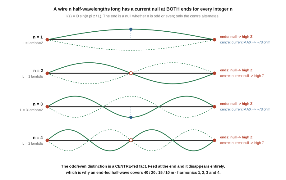
The figure shows where the odd-harmonic folklore actually comes from. Evaluate the same distribution at the wire’s midpoint, z = L/2:
Table 3 — The figure shows where the odd-harmonic folklore actually comes from. Evaluate the same distribution at the wire's midpoint, z = L/2
| n | Length | I(centre)/I₀ | Centre impedance | End impedance |
|---|---|---|---|---|
| 1 | λ/2 | +1.000 | low, ~73 Ω | high |
| 2 | 1 λ | 0.000 | high | high |
| 3 | 3λ/2 | −1.000 | low | high |
| 4 | 2 λ | 0.000 | high | high |
The centre alternates. The end does not. A centre-fed wire presents a low impedance on odd harmonics and a high one on even harmonics, which is precisely why a half-wave dipole fed with coax behaves well on 40 m and 15 m and badly on 20 m and 10 m, and why the multi-band dipole family has to work so hard — see the multi-band dipole dive, where that alternation is the organising problem. Somewhere in the retelling, a true statement about the centre of a wire was carried across to a chapter about the end of one, where it is not merely unhelpful but exactly backwards.
That the distinction vanishes at the end is the end-fed’s real structural advantage, and it deserves to be stated as such rather than left as a correction. A centre-fed wire gets every other harmonic; an end-fed wire gets them all. The 40/20/15/10 coverage that sells these antennas is harmonics 1, 2, 3 and 4 — a consecutive run, not a selection.
One caveat against over-reading this. The end impedance is high on every harmonic; it is not the same high value on every harmonic. §6 takes that up, and it is the reason a four-band antenna shows four different SWR readings even when nothing is wrong with it.
2.4 Which bands actually land
Being resonant at n · f₀ is only useful if n · f₀ falls inside an allocation. The lead figure plots the whole series for the three standard cuts against the US amateur HF bands; the arithmetic behind it is below.
A 40 m cut at 7.10 MHz is the clean case, and it is clean for a reason:
Table 4 — A 40 m cut at 7.10 MHz is the clean case, and it is clean for a reason
| n | Frequency | Lands in |
|---|---|---|
| 1 | 7.10 MHz | 40 m (7.000–7.300) |
| 2 | 14.20 MHz | 20 m (14.000–14.350) |
| 3 | 21.30 MHz | 15 m (21.000–21.450) |
| 4 | 28.40 MHz | 10 m (28.000–29.700) |
Four for four. The fifth harmonic falls at 35.50 MHz, which is not an amateur band anywhere.
An 80 m cut at 3.55 MHz tells a more interesting story:
Table 5 — An 80 m cut at 3.55 MHz tells a more interesting story
| n | Frequency | Result |
|---|---|---|
| 1 | 3.550 MHz | 80 m |
| 2 | 7.100 MHz | 40 m |
| 3 | 10.650 MHz | ✗ misses 30 m (10.100–10.150) by 500 kHz |
| 4 | 14.200 MHz | 20 m |
| 5 | 17.750 MHz | ✗ misses 17 m (18.068–18.168) by 318 kHz |
| 6 | 21.300 MHz | 15 m |
| 7 | 24.850 MHz | ✗ misses 12 m (24.890–24.990) by 40 kHz |
| 8 | 28.400 MHz | 10 m |
Every pre-WARC band lands. All three WARC bands are missed.
A 20 m cut at 14.20 MHz gives 20 m and 10 m, and nothing else: the third harmonic is 42.60 MHz.
2.4.1 Why the misses are structural
The pattern in the second table is not coincidence, and the reason is historical rather than electromagnetic. The traditional HF amateur bands were laid out as a harmonic series on 3.5 MHz — 3.5, 7, 14, 21, 28 are 1, 2, 4, 6 and 8 times 3.5 MHz. A harmonic antenna and a harmonically allocated band plan were made for each other, and the end-fed half-wave’s multi-band trick is in a real sense an artefact of 1920s spectrum policy.
The 1979 World Administrative Radio Conference added 30 m, 17 m and 12 m, and placed them between the existing bands rather than extending the series. They are narrow — 30 m is 50 kHz wide, 12 m 100 kHz — and they sit where no low multiple of 3.5 MHz falls. A harmonic antenna cannot reach them by harmonic action. That is a property of the allocation table, not a defect in the antenna, and no amount of trimming fixes it: shortening the wire to bring the fifth harmonic up onto 17 m drags the fundamental off 80 m and every other harmonic with it.
2.4.2 Do not over-correct: the vendors are not simply lying
It would be easy to end the section there and declare WARC coverage a myth. That would be an over-correction, and the evidence against it is on the vendors’ own pages.
MyAntennas advertises its EFHW-8010 as “Resonant on 80/40/30/20/17/15/12/10m” and “No Tuner Required”. Two things are going on. Real wires do not sit exactly on integer multiples (§5), the SWR minima are broad rather than needle-sharp, and a band that is missed by 40 kHz — the 12 m case — may well be inside the 2:1 skirt of the nearby resonance. And modern transceivers have internal tuners with a modest matching range, so “no tuner required” is a claim about the external accessory rather than about the antenna presenting 50 Ω.
The reviews on that same product page are the citable evidence for how this plays out in the field: one owner reports “Need tuner for 17 & 80m”, another that “Radio internal tuner makes it happy on most all bands.” Both descriptions are consistent with the arithmetic. The honest summary is that an 80 m end-fed half-wave is a genuine no-tuner antenna on the harmonic bands, and a tuner-assisted antenna on the WARC bands — and that a buyer should read “resonant on eight bands” as “usable on eight bands, resonant on five.”
2.4.3 The 6 m claim
The previous edition listed 50–54 MHz as the “5th harmonic” of a 40 m end-fed, at 3.0–5.0:1 SWR. Five times 7.10 MHz is 35.50 MHz. The 6 m band begins at harmonic number 50.00 / 7.10 = 7.04, and the seventh harmonic lands at 49.70 MHz, still 300 kHz below the band edge.
Two separate errors are worth separating, because they have different consequences. The harmonic number is simply wrong, which matters because it is the kind of error that propagates into other people’s tables. The coverage claim is more defensible: end-fed wires frequently do give a workable match somewhere in 6 m, because by the seventh harmonic the wire is nearly four wavelengths long, the impedance excursions are compressed, and a transformer with several picofarads of stray capacitance behaves in ways the simple model does not capture. But that is an antenna that happens to load up, not a resonant harmonic, and it should be described as such. If 6 m matters, the honest advice is to model or measure the specific installation rather than trust a row in a table.
2.5 Why the harmonics do not land exactly
§4 assumed the harmonic resonances sit at exact integer multiples of the fundamental. They do not, and the direction of the error is consistent.
End effect is not a fixed percentage of the wire’s length; it is closer to a fixed physical increment at each end, set by the tip’s capacitance to its surroundings. As n rises, that same physical increment is a larger fraction of the half-wavelength being fitted into the wire, so the fractional shortening required grows with harmonic number. The classic amateur formula for a harmonic wire encodes this directly:
L = 492 · (n − 0.05) / f feet
Solve it for a wire of fixed length whose fundamental is f₁, and the harmonic resonances fall at
f_n = f₁ · (n − 0.05) / 0.95
which is above n · f₁ for every n > 1. Computed for a 40 m cut:
Table 6 — which is above n · f₁ for every n > 1. Computed for a 40 m cut
| n | Integer multiple | End-effect model | Creep |
|---|---|---|---|
| 1 | 7.100 MHz | 7.100 MHz | — |
| 2 | 14.200 MHz | 14.574 MHz | +2.6 % |
| 3 | 21.300 MHz | 22.047 MHz | +3.5 % |
| 4 | 28.400 MHz | 29.521 MHz | +3.9 % |
The direction is reliable and the magnitude is not, and this is the honest limit of the model. Taken literally the table says the second harmonic lands 224 kHz above the top of 20 m and the third 597 kHz above the top of 15 m — and yet these antennas plainly do work on 20 m and 15 m, in very large numbers. The 0.05 constant was derived for bare harmonic long wires, and it over-predicts the creep for a modern end-fed: insulated wire, a transformer with several picofarads of stray capacitance loading the feed end, and heights well below those assumed. No measured set of harmonic resonances for a specific EFHW was available to this volume, so the correct statement is that the resonances creep upward by a few percent, growing with n, by an amount that must be measured on the installed antenna rather than predicted. A per-band resonance sweep on a real wire is one of the bench tasks recorded against this dive.
The practical consequences do not depend on the magnitude, only the direction, and both are things builders actually do:
- Cut for a fundamental at or below the bottom of the lowest band. Everything above it will drift up, so a fundamental placed mid-band puts the top harmonic out of the top of its band. This is why 80 m units are cut for the bottom end of 80 m rather than for the middle.
- Expect the upper bands to sit high in their allocations, and expect the discrepancy to grow with band number. A wire that is spot-on at 7.1 MHz and 400 kHz high on 10 m is behaving normally.
2.5.1 Compensation coils, and what they are actually for
The wire has one length and several bands, so a builder who wants to move one band without moving the others needs a second degree of freedom. The usual one is a small inductor inserted at a chosen point along the wire — a compensation or loading coil, sometimes sold as a “linear loading” element.
The principle is positional. An inductor adds electrical length in proportion to the current flowing through it, so a coil placed where the current is large on one band and small on another affects those bands very differently. The current distribution changes with n (§3’s figure shows exactly how), so a point that sits near a current maximum on the third harmonic may sit near a null on the second. Choosing the position is choosing which band to move.
Two cautions. First, this is a genuinely fiddly optimisation, it interacts with everything else on the wire, and the published designs are the product of modelling rather than of a closed-form rule — AF7NX’s work is the most careful treatment the author found. Second, and to keep this consistent with Vol 1: the compensation capacitor across the primary of a 49:1 transformer is a different device solving a different problem. It compensates the transformer’s own high-frequency behaviour at the top of its range; it does not tune the wire, and it will not move a band. Coil on the wire, capacitor on the transformer — they are frequently confused, and the confusion sends builders to change the wrong component. The build detail for both belongs to Vol 5.
2.6 Why the same wire shows a different SWR on every band
The end impedance is high on every harmonic. It is not the same value on every harmonic, and a fixed-ratio transformer has no way to accommodate that.
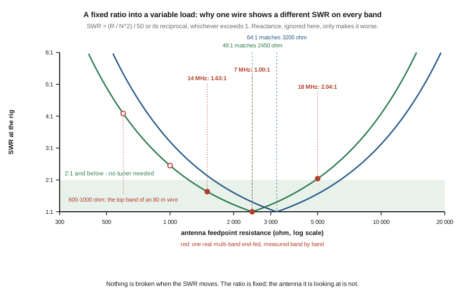
A 49:1 transformer divides whatever resistance it sees by 49. It presents 50 Ω to the rig when, and only when, the antenna presents 2450 Ω. Everywhere else the transmitter sees the mismatch scaled down but not removed:
Table 7 — A 49:1 transformer divides whatever resistance it sees by 49. It presents 50 Ω to the rig when, and only when, the antenna presents 2450 Ω. Everywhere else the transmitter sees the mismatch scaled down but not removed
| Antenna R | Rig sees | SWR |
|---|---|---|
| 600 Ω | 12.2 Ω | 4.08:1 |
| 1 000 Ω | 20.4 Ω | 2.45:1 |
| 1 500 Ω | 30.6 Ω | 1.63:1 |
| 2 450 Ω | 50.0 Ω | 1.00:1 |
| 5 000 Ω | 102.0 Ω | 2.04:1 |
A 49:1 transformer holds 2:1 or better only between about 1225 Ω and 4900 Ω — a four-to-one window. A 64:1 shifts the same window up to 1600–6400 Ω, which is the entire argument for that ratio on longer wires, and is a better description of it than any story about wire Q.
The marked points on the figure are a real multi-band end-fed measured band by band, recorded in the antenna tuners dive: 2450 Ω at 7 MHz, 1500 Ω at 14 MHz, 5000 Ω at 18 MHz. Run through 49:1 those give 1.00:1, 1.63:1 and 2.04:1 respectively — three quite different SWR readings from one wire, one transformer and no fault anywhere. The hollow markers are the other end of the range: for an antenna whose fundamental is 80 m, the feedpoint resistance on 10 m can fall to 600–1000 Ω, which is 4.08:1 and 2.45:1 through the same transformer.
Two things make the real picture worse than the table.
Reactance. The figures above are pure resistance. A real feedpoint is R + jX, and Vol 1 showed that a fixed-ratio transformer scales reactance by the same factor as resistance but cannot cancel it. An antenna 1 % off resonance on some band arrives at the rig still off resonance, with a reactive component added to whatever resistive mismatch it already had. Every SWR figure here is therefore a floor.
Loss flatters the reading. A lossy transformer improves SWR, because power dissipated in the ferrite never reaches the antenna and never comes back as a reflection. This is worth internalising before trusting a flat SWR curve as evidence of a good antenna: the flattest sweep in a comparison may be the worst-performing unit in it. The measurements behind that claim, and the transformer loss figures that put numbers on it, are in Vol 4.
For completeness, the shape a typical 40 m end-fed’s SWR takes across HF, as commonly reported:
Table 8 — For completeness, the shape a typical 40 m end-fed's SWR takes across HF, as commonly reported
| Band | Harmonic | Typical SWR |
|---|---|---|
| 40 m | 1 | 1.3–1.8:1 |
| 20 m | 2 | 1.5–2.5:1 |
| 15 m | 3 | 1.8–2.8:1 |
| 10 m | 4 | 2.0–3.0:1 |
| WARC bands | — | 4–8:1 |
⚠ These specific numbers are inherited from the previous edition and no source was found for them. They are retained because their shape is consistent with everything above — a good match on the fundamental degrading progressively with harmonic number, and the non-harmonic bands far outside the transformer’s window — but they are representative rather than measured, and they are not a specification for any particular product. Measure the antenna you actually built.
2.7 What the pattern does across the harmonic bands
An end-fed half-wave on its fundamental radiates exactly like a centre-fed half-wave dipole. Vol 1 gave the reason: the pattern is set by the current distribution over the whole wire, and the current distribution is a property of the resonant structure rather than of the point you chose to inject power at. A wire carrying a half-wave standing wave produces the classic broadside figure-eight whether it is fed in the middle or at the tip.
On the harmonic bands the wire is one, one-and-a-half or two wavelengths long, the current distribution is different, and the pattern changes with it.
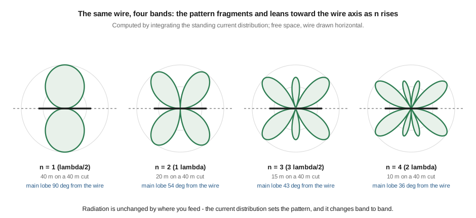
The figure is computed rather than redrawn: for each n, the far field is the integral of the standing current sin(nπz/L) against the propagation phase along the wire, multiplied by the element factor. The resulting main-lobe angles, measured from the wire axis:
Table 9 — The figure is computed rather than redrawn: for each n, the far field is the integral of the standing current sin(nπz/L) against the propagation phase along the wire, multiplied by the element factor. The resulting main-lobe angles, measured from the wire axis
| n | Length | Band on a 40 m cut | Main lobe from the wire | Lobes in the plane |
|---|---|---|---|---|
| 1 | λ/2 | 40 m | 90° (broadside) | 2 |
| 2 | 1 λ | 20 m | 54° | 4, all equal |
| 3 | 3λ/2 | 15 m | 43° | 6 — four at 43°, two broadside 2.9 dB down |
| 4 | 2 λ | 10 m | 36° | 8 — four at 36°, four at 75° and 3.7 dB down |
The computed angles agree with the conventional long-wire table to within a degree, which is a useful confirmation rather than a correction: the previous edition’s figures of 54°, 42° and 36° were right, and the temptation to “fix” them should be resisted. The one enrichment is the lobe count at the fourth harmonic — there are eight lobes in the plane, not four, though only four are major, so describing them as “four major lobes at 36°” was defensible.
What this means operationally is less dramatic than the figures suggest. The lobes are broad, the nulls between them are real but narrow, and at the one-decibel level HF propagation does not care. The practical readings are:
- The wire has a preferred direction that changes with band. Broadside on the fundamental, then progressively more end-fire as you go up. An antenna oriented for a favourite path on 40 m is not oriented the same way on 10 m.
- The nulls off the ends deepen on the fundamental and fragment above it. On 40 m the deep nulls are genuinely off the wire’s ends; by the fourth harmonic the strongest lobes are only 36° off the axis, so the “don’t point it at the DX” advice inverts.
- None of this is pattern control. If the pattern matters — if you are trying to put a null on a specific interferer, or gain on a specific path — the answer is a rotatable directive array, not a wire. The Yagi-Uda dive covers what real pattern control costs and delivers.
All of the above is free space. Over real ground the elevation behaviour is dominated by height, which is the next section, and the azimuth lobing survives roughly intact while the elevation structure is completely rewritten.
2.8 Height, ground and surroundings
For a horizontal wire the single most consequential installation variable is height measured in wavelengths, and a multi-band antenna has a different electrical height on every band it works. That is the fact this section exists to make concrete.
Over ground, the direct ray and the ray reflected from the surface combine, and over a perfectly conducting ground the reflection reverses phase, putting a null on the horizon and the first elevation maximum at
θ = arcsin(λ / 4h)
which has no solution below h = λ/4 — meaning that a wire lower than a quarter-wavelength has no distinct low-angle lobe at all and radiates most strongly straight up. Real ground is lossy rather than perfectly conducting, which fills the horizon null in slightly, softens the lobe structure and costs a decibel or two, but it does not move the maxima much; the angles below are the ideal-ground values and should be read as the shape of the behaviour rather than as a prediction for a specific soil. Take one 10 m mast and a 40 m end-fed on it:
Table 10 — which has no solution below h = λ/4 — meaning that a wire lower than a quarter-wavelength has no distinct low-angle lobe at all and radiates most strongly straight up. Real ground is lossy rather than perfectly conducting, which fills the horizon null in slightly, softens the lobe structure and costs a decibel or two, but it does not move the maxima much; the angles below are the ideal-ground values and should be read as the shape of the behaviour rather than as a prediction for a specific soil. Take one 10 m mast and a 40 m end-fed on it
| Band | λ | Height | First elevation maximum |
|---|---|---|---|
| 40 m | 41.9 m | 0.24 λ | no lobe — straight up (NVIS) |
| 20 m | 21.2 m | 0.47 λ | 32° |
| 15 m | 14.1 m | 0.71 λ | 21° |
| 10 m | 10.5 m | 0.95 λ | 15° |
The same wire on the same mast is a near-vertical-incidence antenna on its fundamental and a low-angle DX antenna on its top harmonic. This is the correct explanation for the most common report about these antennas — that they are “great on the high bands and only good for close-in work on 40” — and it is not a property of the end-feeding, the transformer or the harmonic operation. It is height. A dipole at the same height does the same thing. Anyone diagnosing an end-fed’s performance should establish the electrical height on the band in question before reaching for any other explanation.
The corollary is that the trade-off is real and not always the one you want. Getting 40 m off the ground electrically means a 10 m mast becoming a 20 m mast, which is a different class of installation. In practice most owners accept a compromise, and the compromise is usually chosen — knowingly or not — by which bands they care about.
2.8.1 Surroundings, and where the antenna is sensitive
The end-fed’s sensitivity to nearby objects is not uniform along the wire; it is concentrated where the voltage is high.
- The far tip is a voltage maximum on every band. Bringing it close to a gutter, a wet tree limb, a metal fascia or a downpipe loads it capacitively, shifts every resonance down and, at power, invites arcing and dielectric loss in whatever is doing the loading. The end insulator is a high-voltage RF component and the rope beyond it should be a decent length of non-absorbent line.
- The feed end is also a voltage maximum, and it carries the transformer, the enclosure and the coax connector. This is §2’s point restated: the hardware is part of the antenna and its stray capacitance is not negligible.
- The middle of the wire is comparatively tolerant on the fundamental, where it is a current maximum and a low-impedance point. It is less tolerant on the harmonics, where §3’s distributions put voltage maxima at intermediate points along the wire too. A wire running close to a metal roof at its midpoint may behave on 40 m and misbehave on 15 m for exactly this reason.
- Sloping the wire, or bending it into an inverted-L, changes both the pattern and the feedpoint, generally raising the radiation angle in one plane and mixing in vertical polarisation. That is a large enough topic to have its own home: Vol 3 covers slopers and inverted-Ls, and it applies to resonant end-feds as much as to the non-resonant wires it is otherwise about.
A last note on expectations, in the same spirit as Vol 1’s note about counterpoises. None of the above will show up as a dramatic difference on a signal report, because HF propagation is a noisy channel and a few decibels of takeoff-angle change is not visible in a single QSO. It shows up statistically, over weeks, as which paths the antenna does and does not work — and it shows up immediately on a NanoVNA as a change in where the resonances sit.
2.9 Where this volume hands off
The resonant end-fed half-wave is now specified. It is cut a few percent short of a free-space half-wave, at a length that must then be trimmed against the actual installation. It is resonant on every integer harmonic, not the odd ones, which is the source of its consecutive multi-band coverage. Those harmonics land inside the pre-WARC bands because the pre-WARC bands were allocated as a harmonic series, and they miss the WARC bands because the WARC bands were deliberately placed off it. The resonances creep upward with harmonic number by a few percent, so the fundamental is cut low. The SWR differs on every band because a fixed transformer ratio is looking at a feedpoint resistance that moves by nearly an order of magnitude across the range. The pattern fragments into progressively more, progressively more end-fire lobes. And the elevation behaviour on any given band is set by height in wavelengths, which for a multi-band antenna is a different number on every band.
From here:
- Vol 3 — Non-resonant wires leaves the harmonic series behind for the random wire, the long wire, the inverted-L and the sloper: why “random” is not arbitrary, which lengths to avoid and why, and the 9:1-plus-tuner system as a different design philosophy rather than a cheaper version of this one. The end-fed long wire — longer than a half-wave, with its higher feedpoint impedance and its 64:1 or 81:1 transformer — belongs there too.
- Vol 4 — Feed, counterpoise and the ground question picks up every thread this volume deferred to a measurement: the transformer selected against a measured impedance rather than an assumed one, the loss that flatters an SWR sweep, counterpoise length in the field, and common-mode current as the second device in the system.
- Vol 5 — DIY build, measurement and buys cuts and trims a real wire with a VNA, works through the compensation-coil question at build level, and surveys what is worth buying — including how the trade rates these antennas by duty cycle rather than by a single wattage.
Three items are owed against this volume and are recorded rather than quietly skipped. A measured set of harmonic resonances for a specific end-fed would replace §5’s over-predicting model with real numbers, and is a bench task rather than a literature one; the NanoVNA dive has the method. The SWR figures in §6 are inherited and unsourced, and are flagged in place. And the figures in this volume were generated numerically and verified against their formulas but not rendered by a browser at authoring time, so they are on the pre-publish check list.
2.10 Resources
- ARRL band plan and 47 CFR §97.301 — the allocation edges every harmonic in §4 is measured against. The misses are computed against the band edges themselves, not against a nominal band centre.
- AF7NX, Engineering the EFHW 49:1 Transformer and Antenna (Squash Practice, 2021) — the stray-capacitance measurements behind §2, the compensation-coil work referenced in §5, and the NEC study this dive leans on throughout. The most careful single treatment of this antenna the author found.
- MyAntennas EFHW-8010-1KW-ICAS product page — the source for the WARC coverage claim in §4 and, in its own review section, for the two owner reports that qualify it. A useful reminder that vendor pages sometimes carry their own best counter-evidence.
- ARRL / HF Kits End-Fed Half-Wave Antenna Kit documentation — the canonical 40 m cut at about 66 ft for 40/20/15/10 m.
- Vol 1 — Why end-feeding works at all — the standing wave, the
R(z) = 73/cos²(βz)derivation behind §6’s variable feedpoint, and the reciprocity argument about counterpoises. - Multi-band dipoles, Vol 1 — the same harmonic problem seen from the centre of the wire, where the odd/even alternation of §3 is a genuine design constraint.
- Yagi-Uda, Vol 2 — what actual pattern control costs, for the reader who reaches §7 and wants more than lobes.
- Antenna tuners, Vol 1 — the per-band feedpoint impedance set plotted in §6.
- NanoVNA, Vol 4 — the measurement technique for the resonance sweep this volume asks for and does not have.
Comments (0)